Goal: Mutual Information is an interesting quantity as it measure correlations between data which cannot be measured by the correlation function. The goal of this project is to develop a general enough implementation of mutual information which can be applied to any kind of data, and then to explore how to extract meaningful measurements from different types of data.
Results: We were able to develop a function which calculates mutual information between two sets of data, and relies on a distance function to do so. As any data can be considered to be embedded in a metric space, this implementation works in principle for any kind of data, whether it is images, videos or just time series. We then tested and later explored how this can be used for extracting meaningful measurements from audio and videos of well known systems, and ultimately applied it to a more general example.
Further developments: The function uses a k-th nearest neighbours approach to estimate mutual information, so heavily relies on built-in functions like Nearest and DistanceMatrix. Efficiency is certainly an issue that must be addressed, especially when using user-defined distances compared to built in ones. Furthermore, exactly which distance or preprocessing is useful in extracting meaningful measurements is an open ended question which needs much more investigation.
Imagine you’re sitting by a fountain looking at the calming and steady movement of the water stream going up and down. Then a thought strikes: is it just a periodic movement, or is there something more? Say you just have a camera and record the movement to inspect it later out of curiosity.
To extract something even remotely meaningful would require quite a bit of image processing on the video frames, an expert’s work. What if you had a function which allowed you to just plug in the video and get an estimate, even if a bit rough, of how much information is “common” to the frames? And what about doing the same with, say, the frequency spectra or the amplitude of an audio file?
The approach we explored in this project is to implement a function which estimates a quantity called mutual information. Consider two random variables and , the mutual information is a quantity which tells how much information about we can get by observing . More precisely, if we consider the Shannon entropy , the mutual information is defined as:
X
Y
I(X,Y)
X
Y
H(X)
I(X,Y)=H(X)-H(X|Y)
where is the entropy of conditioned on . It is common in information theory to interpret the Shannon entropy as a measure of the “uncertainty” of a random variable, thus from the above formula we can interpret the mutual information as the amount of uncertainty which is removed from when observing .
H(X|Y)
X
Y
X
Y
But what has this to do with media files? Well, pretty much any media file can be thought as laying on some kind of metric space, i.e. a space with a distance function. Once one has a distance between two objects, one can devise a procedure to “bin” the space they lay in and look at them as probability distributions.
More in detail, we implemented an estimator published by Kraskov et al. , which relies on general enough assumptions about the two variables and , which in turn allowed us to apply it to any kind of numeric data or file by just making use of built-in or user-defined distance functions.
X
Y
In the following, we will sometimes refer to the mutual information as MI.
Example : Logistic Map
Example : Logistic Map
But why should we care about the mutual information? There are many other quantities which are able to estimate relationships among variables and which are easier to compute, like for example the widely used correlation function. The point in using the mutual information is that it can detect relationships of higher order than the correlation function does. In particular, if we briefly go back to random variables, the mutual information becomes 0 if and only if the two variables X and are totally independent from each other, or in other words:
Y
I(X, Y) = 0 ⇔ =·
p
XY
p
X
p
Y
where is the joint probability distribution of the two variables and . This is a property which the correlation function doesn’t have, and in particular it is well know that it can be zero even when the two variable share a quadratic dependence.
p
XY
X
Y
In order to better illustrate the concept above, let’s consider a well know system: the logistic map, a 1D system which for some parameter values exhibits chaotic motion. Its evolution is given by the iterations (on an initial condition ∈[0,1] ):
x
0
x
n+1
x
n
x
n
It is clear that the function above has a quadratic form:
In[]:=
Manipulate[Plot[rx(1-x),{x,0,1},PlotLabelStyle[(r)(1-),14,Bold],AxesLabel{"x"}],{{r,4.},0.,4.,0.1}]
x
Style["n",Italic]+1
x
Style["n",Italic]
x
Style["n",Italic]
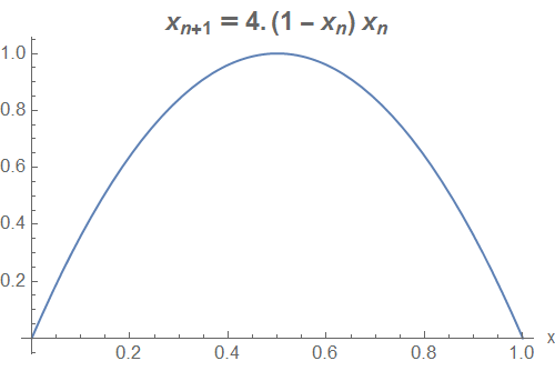
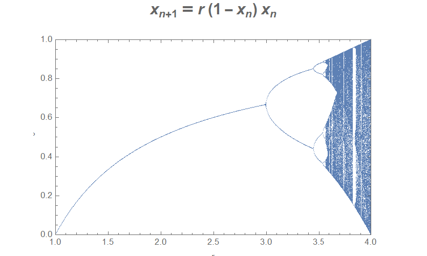
If we iterate the function it will eventually end up cycling between a set of values or even just a single one. This set is called an attractor.
In the plot below we show the attractor of the logistic map as a function of the starting point and the rate (credits: wolfram demonstration project): what’s interesting is that after r≈3.56995 the attractor actually comprehends an infinite set of points.
In the plot below we show the attractor of the logistic map as a function of the starting point
x
0
r
In[]:=
Manipulate(limits=Compile[{r},({r,#1}&)/@Union[Drop[NestList[#1r(1-#1)&,0.234,pts],300]]];)bifurcation[r0_,r1_,n_]:=FlattenTablelimits[r],r,r0,r1,,1;ListPlotbifurcation[beginr,If[endr<4,endr,4],pts],PlotStyleAbsolutePointSize[0.1],SequenceAxesOrigin{beginr,ylow},PlotRange{{beginr,If[endr<4,endr,4]},{ylow,yhigh}},FrameLabel{"r",""},PlotLabelStyle[(r)(1-),18,Bold],ImageSizeLarge,FrameTrue,ImagePadding20,TicksRangebeginr,If[endr<4,endr,4],(If[endr<4,endr,4]-beginr),Range0,1,Ifyhigh-ylow<0.3,,0.1,Grid[{{Control[{{beginr,2.9,"beginning r"},1,3.9999,0.01,ImageSizeSmall,Appearance"Labeled"}],Control[{{yhigh,1,"high end of y axis"},0.01,1,0.01,ImageSizeSmall,Appearance"Labeled"}]},{Control[{{endr,4,"ending r"},2.9,4,0.01,ImageSizeSmall,Appearance"Labeled"}],Control[{{ylow,0,"low end of y axis"},0,0.99,0.01,ImageSizeSmall,Appearance"Labeled"}]}},AlignmentRight],{{pts,600,"number of points"},600,3000,300,Appearance"Labeled"},TrackedSymbolsTrue,SynchronousUpdatingFalse
r1-r0
n
x
0
x
Style["n",Italic]+1
x
Style["n",Italic]
x
Style["n",Italic]
1
5
yhigh-ylow
10
What about the correlation between consecutive points in the evolution of the map? In the plot below, we show how the correlation function rapidly plunges to 0 after just one step, whereas the mutual information decreases much more slowly, for .
r=4
In[]:=
ClearAll[lm];lm=Compile[{{x,_Real},{r,_Real}},NestList[r*#(1.-#)&,x,10000]];Block[{mutinfo,logdata,corr,root,timeMI,timeCorr,mivalue,r=4.},logdata=lm[RandomReal[],4.];{mutinfo,corr}=Transpose@Table[{KraskovI1[logdata〚;;1000〛,logdata〚(T+1);;(1000+T)〛,4],CorrelationFunction[logdata〚;;1000〛,T]},{T,0,20}];ListLinePlot[{mutinfo,corr},PlotRangeAll,PlotLabel"Mutual Information vs Correlation",Epilog{Inset[LineLegend[ColorData[97]/@{1,2},{"Mutual Information","Correlation"}],Center]},AxesLabel{"Time"},ImageSizeLarge]]
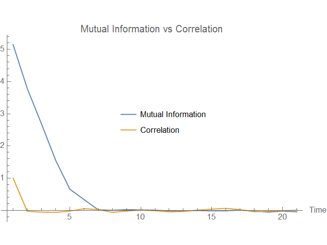
This means that the mutual information shows a relationship between consecutive points which cannot be seen by the correlation function.
Application: delay embedding of Rössler attractor
Application: delay embedding of Rössler attractor
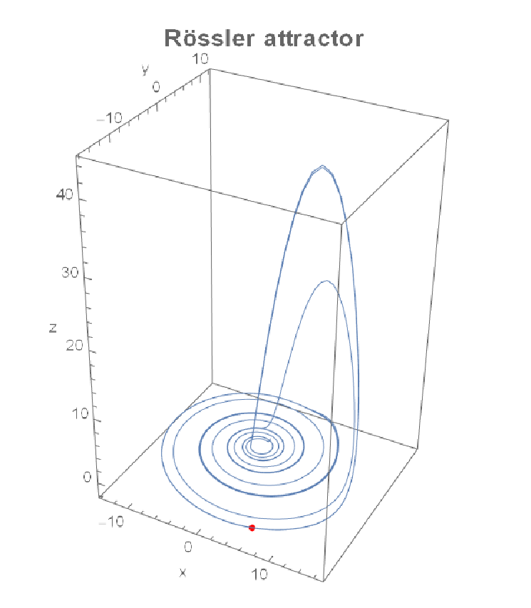
In order to test our implementation of the mutual information, we then decided to apply it to another system. We took into consideration the Rössler attractor, defined by the equations
x'=-y-z |
y'=ay+x |
z'=b+z(z-c) |
The solutions to the above system gives the attractor represented below:
ClearAll[rosslervalues];Module[{x,y,z},rosslervalues=With[{a=0.2,b=0.2,c=8.0},NDSolveValue[{x'[t]-(y[t]+z[t]),y'[t]x[t]+ay[t],z'[t]b+x[t]*z[t]-cz[t],x[0]1,y[0]1,z[0]1},{x,y,z},{t,0,10000}]];Manipulate[Show[ParametricPlot3D[Through[rosslervalues[t]],{t,0,100},PlotRangeAll,PlotLabelStyle["Rössler attractor",16,Bold],AxesLabel{"x","y","z"},PlotStyle{Thin},ImageSizeLarge],Graphics3D[{Red,PointSize[Medium],Point[Through[rosslervalues[time]]]}]],{{time,0,"Time"},Range[0,100,0.1],ControlTypeSlider},SaveDefinitionsTrue,SynchronousUpdatingFalse]]
Now, we want to use the mutual information to perform delay embedding. Basically, say I have the above system but can only measure the first coordinate x(t), at certain time intervals. Can I reconstruct the system properties just from it?
We see that the shape above is quite close to the initial one, apart from a smooth geometrical transformation.
In the plot below, we show our estimation of the mutual information for this system. The minimum seems close to ≈1.5s (time scale must be divided by 10)
We also computed the correlation, using the built-in function CorrelationFunction, and compared it in the plot with the mutual information. Notice that their oscillations are similar, but the peaks in the latter are a clearer indication of the periodic behavior of the Rössler attractor. In particular, the second peak corresponds to a full period, and the first minimum is expected to be somewhere a quarter of the period.
The behaviour we get is quite similar to the expected one, but now another question arises. Does this estimator for MI depend on the particular distance used?
We talked before about using different distances, and until now we' ve used the so called ∞ - norm under the hood (ChessboardDistance in Mathematica), but any distance function can be easily plugged in the MI estimator just by using the DistanceFunction option and providing either a built-in or a user defined function (here for simplicity we plot on a shorter timescale):
We can clearly see from the plots above that, for such a simple system, the behaviour is the same no matter which distance function is used.
Applications: audio and video
Applications: audio and video
Ok, everything seems to be good on well know systems, but why do we not pass to something a bit more interesting? Let' s say I have an audio or video file of any kind, can I extract some information from it in a way I can make sense of it?
In principle, any list of “stuff” can be plugged into the MI estimator. But in order to extract some useful information, we must be careful about what we actually feed to it.
Audio
Audio
Let' s consider again the Rössler system, but this time in a slightly different setup. We encode its first coordinate in an audio file using midi tones:
The audio is funny, but the spectrogram is quite interesting too (we applied a LowPass filter to filter out noise at higher frequencies):
It would be nice now to recover the behaviour we saw above for the Rössler attractor just from the frequency spectra of this audio file. But we first need some kind of distance on frequency spectra! We’ll use two different distances:
Now we just have to plug into the MI estimator the frequency spectra and the distances:
The behaviour obtained is strikingly similar to the Rössler original one! Also, once again we get similar results for two different distances. The exact values obtained depend on the sampling rate of the audio and on how we encode the values into frequency, but the functional form doesn’t lie.
Video
Video
Since we' ve briefly touched audio, the next step is video files! Let’s consider this animation of a double pendulum:
What's its information content? We can compute the mutual information from its components:
How can we extract the same estimation from the animation above? We attempted in many different ways. In particular, we noticed that just using DimensionReduce in 3 dimension gave an interesting result:
Using the "TSNE" method just on the list of frames, we get quite a nice trajectory. If we plug the data points obtained into our estimator:
Through this procedure, we get a behaviour which is quite similar to the estimation of MI on the first pendulum coordinate! Since the frames contain both pendulums, a small contribution from the second pendulum can be seen from the fact that the valleys and the sixth peak are a bit higher than in the first pendulum MI.
Karman vortex street
Karman vortex street
Until now we’ve seen some example of system we were able to reproduce entirely through some system of differential equations. What about a system of which we do not know the behaviour beforehand?
An interesting one is the Karman vortex street: imagine having a fluid flowing in one direction and a fixed obstacle is in the way. If the fluid flows at low speeds it will mostly just go around the obstacle without much hassle, but as the speed increases (typically with Reynold's number ⩾ 90) vortexes will start forming from the obstacle and will be transported along with the flow, forming kind of a path. The video below shows a (simulated) example of what we just described:
An interesting one is the Karman vortex street: imagine having a fluid flowing in one direction and a fixed obstacle is in the way. If the fluid flows at low speeds it will mostly just go around the obstacle without much hassle, but as the speed increases (typically with Reynold's number ⩾ 90) vortexes will start forming from the obstacle and will be transported along with the flow, forming kind of a path. The video below shows a (simulated) example of what we just described:
We can see that in this particular video there’s a quite repetitive and regular behaviour. We tried following the same procedure as for the double pendulum, by using DimensionReduction on the frames to 3 dimensions, with the TSNE method (we also trim to the interesting part):
The results are quite interesting: there’s a clear periodicity in the plot, with just a bit of noise. Notice that we had to convert the frames to grayscale in order to use DimensionReduce.
Let' s try to see if we can extract some indication of this behaviour from the MI estimator:
We see that the mutual information initially goes down, but then plateaus to a constant value, quite a high value compared to the other plots we’ve seen until now. We interpret this as an indication of the highly regular behaviour of the system shown in the video above: a high value of the mutual information indicates high predictability in the system evolution.
But as the system evolves one might expect to see, every few frames, some prominent peaks indicating the period of the system. We weren’t able to see any clear peak from the method above, so we attempted another approach: since the vortexes create a distortion in the background colors, maybe trying to follow such a distortion on the image might work. We used ImageKeypoints with a maximum of 30 markers:
Now we have just what could be seen as a distribution of points in 2D, for every frame. If we apply the MI estimator to this distribution:
The absolute value of the MI is quite off with respect to the previous graph, but what we think is interesting in the above plot is that every two peaks we get exactly the same frame, so that every other peak corresponds to the creation of a vortex. The mean frame distance between two consecutive peaks is about 6.25 frames, so we estimate to see a new vortex every 12-13 frames.
Conclusions and further work
Conclusions and further work
We have implemented a function which computes mutual information and is general enough to be applied, without much thinking behind, to any kind of data, from numeric vectors to video and audio. We applied it to well known systems in order to check its behaviour, which turned out to be consistent with the expectations.
We later tried to answer the question whether patterns in media file could be extracted using this estimator. We first restricted to media files related to well known systems of which we had a functional form to compare and obtained close results, which encouraged us to try exploring an unknown system such as the Karman vortex street.
Many questions remains open: in particular, for the case of video data we attempted to just apply the estimator to list of images (with no preprocessing or conversion), and computed the MI using just ImageDistance with various options. This gave decent results on videos with a uniform background (which we unfortunately cannot show), though not so much on the video shown above for the Karman vortex. Due to time constraint and efficiency issues, we couldn’t try many distances on images, so the question of which distance between images might be the best in order to detect different features within frames remains open. On more general terms, the best distance to choose between any kind of data highly depends on what one is looking for, and the question on how to determine it remains an open issue [2].
Also, efficiency issues are to be addressed, especially since they’re connected to what was said above. In fact, using built-in distance functions between numeric vectors usually results in a reasonable running time (also considering that errors are estimated on sub-samples, thus require many runs of the same estimation), but this situation worsen considerably when using user-defined functions for which Nearest and DistanceMatrix are not optimized.