Relativistic mass transformations for topological obstructions in hypergraphs/causal graphs
Tom Lee
University of Bonn
Tom Lee
University of Bonn
Abstract: project description
Relativistic transformations modify the causal graph foliation in time coordinate, and different casual graph updating order gives change on topological obstruction in a (hyper)graph.
So by using explicit computational experiments we investigate how the number of vertices/edges changes of topological obstruction in a given Lorentz transform starting from the rewriting rules that gives simple causal graph structure and furthermore particles/obstructions given by non-planar subgraphs for Wolfram model rules.
Introduction & Computational Simulation
Introduction & Computational Simulation
In Wolfram Model there is an introductory description about the relativistic transformation which is interpreted as foliation update of the causal graph. [1], [2]
Based on those analogy/definitions, we do empirical investigation about the change of updating number of the hyper graph evolution with different structure of causal graph by given Lorentz boost.
Furthermore one can find the relation between the Lorentz factor, γ in discrete Wolfram spacetime model, and cross edge density variation when we apply new updating order of causal graph based on Lorentz transformed foliation.
The general analysis proceses of the research can be summarized as Fig. 1.
Out[]=

Fig. 1 Analysis framework
The first step of the framework is defining the integer coordinate of each node in causal graph, and simultaneously the foliation should represents the initial frame.
Then we can do relativistic boost on space, time coordinate of the each node, and this shift gives new foliation of the causal graph.
For the last step, we apply the new updating order of causal graph back to the original initial condition, then we can get new evolution hyper graphs with same rewriting rules.
Therefore our project purpose can be sum up as,
1. Define the arbitrary causal graph initial frame coordinate of each node and foliation
2. Find relation between Lorentz factor(γ) and the updating number of the hyper graph evolution in discretize Wolfram model space time coordinate
3. Check the convergence of discretize Lorentz factor(γ) by increasing the initial causal graph node number(N)
4. Find relation between the discretize and continuum Lorentz factor(γ) difference and the β(v/c, in our case c=1)
Then for the first step, let us define the key physical concept which are frequently used in Wolfram model/ and this research.
I. Hyper/casual graph and foliation
I. Hyper/casual graph and foliation
The casual graph is simply the graph which has one-directed flow between any two point of the graph.
One can see the example of causal graph in Fig.1, and there is a red line which divide the graph in multiple region. This red lines are call foliation of the graph.
To be specific for the definition of the Causal graph, from the first foliation region, let us call these region as class 1, class 2, class 3 and so on. Then the property of the casual graph is there is no node which has directed edges to the upper class (eg. there is no directed edges from class[i] to class[j], when i>j).
Thus in physics, we can interpret this hyper graph as a generation of the classes, such as class 1 generate class 1, and class 2 generate class 3 and so on. So if we assume each node represent the single event, the new update for each foliation class can represent the "time flow", and this gives us the property of causality.
Out[]=
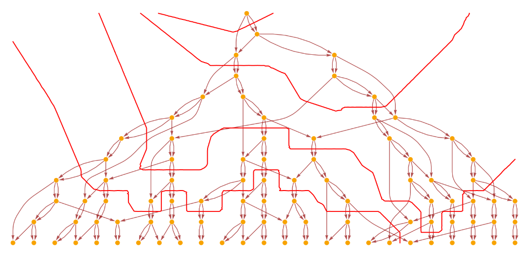
Fig. 2 Example of Causal hyper graph and arbitrary foliation, taken from [1]
Therefore in our models, the concept of time is basically corresponds to the progressive updating of the hypergraph.
For example, the Fig. 3 has the simple structure compare to other general rewriting rules, and it is called as the (triangular) simple causal graph. Here the foliation is noted as red lines and also represents rest frame.(which the foliation line are denoted as parallel horizontal line.)
For example, the Fig. 3 has the simple structure compare to other general rewriting rules, and it is called as the (triangular) simple causal graph. Here the foliation is noted as red lines and also represents rest frame.(which the foliation line are denoted as parallel horizontal line.)
Out[]=
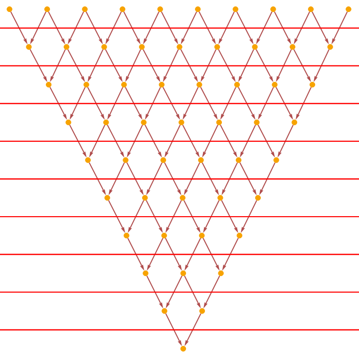
Fig. 3. Example of simple causal hyper graph, taken from [1]
Then from now let us discuss about one rewriting rules that gives the simple casual graph.
RulePlot[ResourceFunction["WolframModel"][{{x,y,y},{y,z}}{{x,y},{y,z,z}}]]
Out[]=
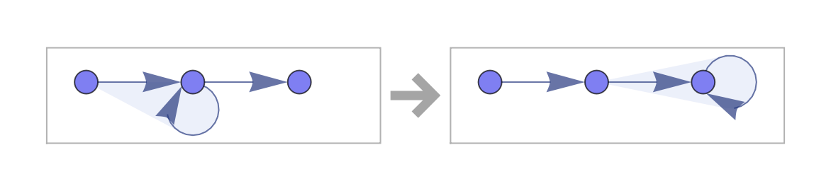
Fig. 4. Example of Rewriting Rule generates simple causal graph, taken from [1]
And by using Wolfram Resource function, we can find which causal graph is generated by this rewriting rule after infinite amount of time. As a result we can get Fig. 5 and this is simple causal graph.
Out[]=
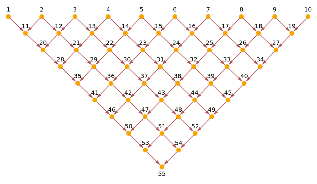
Fig. 5. The causal graph from rewriting rule in Fig. 4
Based on Fig. 5, we can see the hyper graph evolution as Fig 6. In the case of simple causal graph, we do not lose the generality if one assume the initial frame foliation as Fig.3, which has 11 steps of updating.
WolframModel[{{x,y,y},{y,z}}{{x,y},{y,z,z}},toState[StringJoin[Table["BA",10]]],13,"StatesPlotsList"]//Column
Out[]=











Fig. 6. Evolution graph from rewriting rule in Fig.4,, taken from [1]
II. Lorentz Transformation and mass in Wolfram Model
II. Lorentz Transformation and mass in Wolfram Model
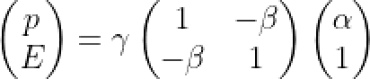
Next in our model, the Energy of the system, E(β) is define as the crossing edge density between causal graph and temporal foliation line. also the momentum of the system, p(β) is the crossing edge density between causal graph and spacial foliation line.
This relation can be written as following matrix multiplication, where α is the spacial distance of the node, and 1 is the temporal distance of the node. So the "crossing edge density"(average distance between each nodes) for each spatial and temporal direction is given as p and E.
This relation can be written as following matrix multiplication, where α is the spacial distance of the node, and 1 is the temporal distance of the node. So the "crossing edge density"(average distance between each nodes) for each spatial and temporal direction is given as p and E.
Out[]=
And to do Relativistic transform of the simple causal graph, let us consider the simple causal graph with initial node number (N)=3 case.
Out[]=
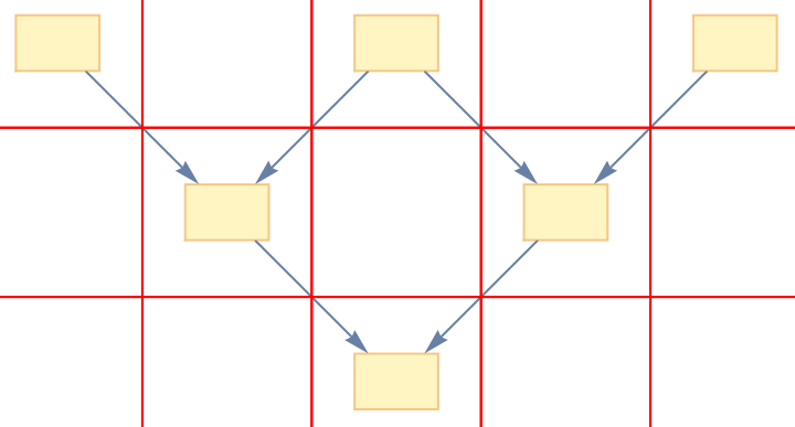
Fig. 7. Initial frame causal graph coordinating, horizontal line is spatial and vertical is temporal line, taken from [1]
As we mentioned, in Wolfram hyper graph model, the each node of the causal graph can be regard as "event". And each "event" has its space and time coordinate, so the coordinating is important to define which line is going to be the foliation of initial frame on arbitrary causal graph. (In this case, we assume the time as being vertical, and space as horizontal direction as default.)
Therefore in case of simple causal graph, in the rest frame which the system speed is zero, the each point should have integer spatial coordinate (eg. -8, -4, 0, 4, 8) and also the temporal coordinate (eg. 0 ,2, 4, 6, 8).
*One can refer more details in the newly defined function simplecausaldata[size_] which generating the coordinated simple causal graph data.
Out[]=
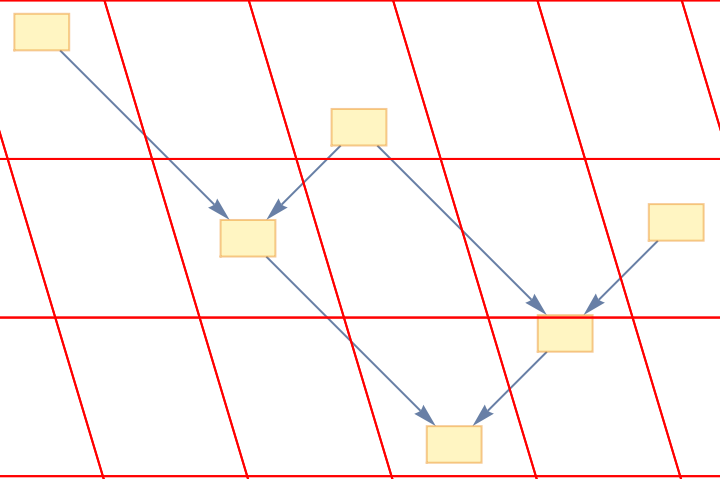
Fig. 8. Lorentz boost result of the each node, here β=0.3, taken from [1]
And after define the coordinate of the each node of initial frame causal graph, it is straight forward to do Lorentz transformation of each event without destroying the causal network, (coneserve straight lines) we can transform a point {t, x} to : [γ(x-β), γ(-βx+t)], which gives Fig. 8 as a result.
Here we can see that Fig.8 has different foliation of the graph compare to Fig. 7, such as event 1, 2, 3 is not happen in same time after relativistic boost.
Thus as one could see here, to do Relativistic transform of the causal graph, there is important process should be done priory. The initial frame coordinating, which is important to define where is the foliation line of initial frame on arbitrary causal graph. And at this point, this is not complete form of the definition, however we can briefly define several step of the coordinating rules in initial frame as following.
[1] Each node should pace in integer point in spacial coordinate.
[2] For each evolution step, the even(graph note)distribution in spacial equally because there is no preference for specific event.
[3] In (j)th causal graph update, if there is k-new node(which does not have causal edge form (j-1)th update step) is generated, then these new node can overlap with other original nodes(which has causal edge connection with previous update).
The further definition of the initial frame definition need more detail investigation.
In general, with many initial node causal graph case, for example N=10,one can get Fig. 9 as a result after the boost. In the same way, for each node space-time coordinate one can adjust the Lorentz transformation with speed β=0.3 (c=1)
Out[]=
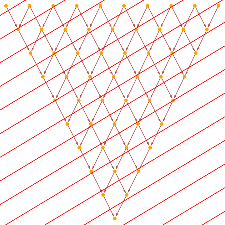
Fig. 9. Example of Lorentz transformed simple causal graph, taken from [1]
Also with new foliation in Fig. 9, we can get Fig. 10 as result of hyper graph evolution. As expected we can get more update step=14, which means the momentum is increased compare to initial frame.
Then how should we interpret this in physical view? As we discussed in our model, the momentum of the system p(β) is the crossing edge density between causal graph and spacial foliation line. So empirically we can assume that when the updating number on evolution graph is increase, then there is more crossing edges are produce. So it can interpret as Lorentz factor multiplier on momentum in continuum physics. Therefore we can safely assume that the Relativistic phenomenon is indirectly observe in Wolfram Model by using the Causal graph transformation and the size of update number in evolution graph.
Then how should we interpret this in physical view? As we discussed in our model, the momentum of the system p(β) is the crossing edge density between causal graph and spacial foliation line. So empirically we can assume that when the updating number on evolution graph is increase, then there is more crossing edges are produce. So it can interpret as Lorentz factor multiplier on momentum in continuum physics. Therefore we can safely assume that the Relativistic phenomenon is indirectly observe in Wolfram Model by using the Causal graph transformation and the size of update number in evolution graph.
p_Lorentz = γ p_initial is equivalent to,
(updating number of hyper graph at initial) = γ_dsic (updating number of hyper graph after relativistic boost)
(updating number of hyper graph at initial) = γ_dsic (updating number of hyper graph after relativistic boost)
Fig. 10. Evolution graph with new foliation updating rule of Causal graph, β=0.3, taken from [1]
Results
Results
I. Example (1) Triangular Simple Causal Graph
I. Example (1) Triangular Simple Causal Graph
For the simplicity, let us consider the rewriting form which have simple casual graph, and also have localization represent as a ring. Then first, without the Lorentz boost, there is 11 hyper graph evolution (update number) is generated.
Fig. 11. Ring structure hyper graph evolution, initial frame
The Fig. 12 shows the Causal graph structure of the hyper graph evolution, and it is identical to simple causal graph.
So we can adjust same analogy for Lorentz boost foliation which is discussed in previous sections.
So we can adjust same analogy for Lorentz boost foliation which is discussed in previous sections.
Fig. 12. Causal graph of the ring structure hyper graph evolution in Fig. 11 , it is same as Fig. 5
Moreover, for the analysis convenience, we make a new function which make the automate for simple causal graph coordinating, Lorentz transformation of each node, and the classify the each node with different foliation-class.
New Functions
New Functions
The first new function is "simplecausaldata[size_]", and it works as coordinating the simple causal graph. It generate the data table of each node. For example {1,0,3} means node number 1 is at (0,3) coordinate on (time, space) order.
The second function "Foliationclass[data_]" is work classify the each node into same range of time, for example -1 to 1, 1 to 3, etc. Then one can see which nodes are in same time range, moreover can see the causal network of the nodes.
The second function "Foliationclass[data_]" is work classify the each node into same range of time, for example -1 to 1, 1 to 3, etc. Then one can see which nodes are in same time range, moreover can see the causal network of the nodes.
Fig. 13. Ring structure Causal graph with Lorentz boost, β=0.3
As a result, we can generate hyper graph evolution with newly updated foliation when β=0.3 in Fig. 13.
There is 14 hyper graph evolution (update number). This is larger than initial case, 11, so satisfy the lorentz boost effect on momentum, p.
Then next question we can ask is "Does this updating number is effect by the initial node number (N) of the causal graph?"
To analyze this, one can make "ratio[n_,beta]" function which automatically calcualte the ratio between [Updating number of Lorentz frame evolution graph]/[Updating number of initial frame evolution graph].
And let us define this value as γ_disc, so in our case, at β=0.3, γ_disc=14/11=1.28
Fig. 14. β=0.1, γ_disc graph when N is increase. One can see there is convergence when N is increasing.
Fig. 14 shows the β=0.1 case of γ_disc graph. The black line is the converge value of the discrete Lorentz factor, and the blue line is the theoretical Lorentz factor at continuum limit.
Then this converging behavior is also appear in different Lorentz boost velocity?
Then this converging behavior is also appear in different Lorentz boost velocity?
Fig. 15. β=0.3, γ_disc graph when N is increase. One can see there is convergence when N is increasing.
Fig. 16. β=0.5, γ_disc graph when N is increase. One can see there is convergence when N is increasing.
So by Fig 14 to 16, we can see convergence behavior for different boost velocity.
And interestingly (rather it is just empirical assumption), it seems there is convergences values for every boost velocity between 0 to 1.
Then now we can think about, "if for each β value there is converging value for γ_disc, then this converging value have some kind of relation with the β?"
To answer this question, let us first define γ_{disc,conv} as a convergence value of γ_disc at each velocity.
Fig. 17. The linear relation for γ_{disc,conv} / γ_cont ratio and boost velocity in simple causal graph. (c=1, v=β)
Finally we can get Fig. 17 as the result for γ_{disc,conv} / γ_cont ratio when boost velocity is increase. (c=1, v=β)
The fitting of the data point is close to linear function, which have y-intercept at 1.
This is quite interesting result because if we define ,
The fitting of the data point is close to linear function, which have y-intercept at 1.
This is quite interesting result because if we define ,
Then we can get following relation.
Here "a" is 0.96 in triangular simple causal graph case, in 2 dimension.
So it menas the Lorentz factor error ratio
Then we can ask again that, this is just for simple causal graph case, or general properties in arbitrary causal graph structure?
To answer this, let us consider another simple hyper graph, call Grid-like causal graph.
So it menas the Lorentz factor error ratio
Then we can ask again that, this is just for simple causal graph case, or general properties in arbitrary causal graph structure?
To answer this, let us consider another simple hyper graph, call Grid-like causal graph.
II. Example (2) Grid-like simple Causal Graph
II. Example (2) Grid-like simple Causal Graph
For the simplicity, the rewriting is same with simple casual graph case, and initial condition also have localization represent as a ring.
Then without the Lorentz boost, there is 4 hyper graph evolution (update number, without periodicity).
Then without the Lorentz boost, there is 4 hyper graph evolution (update number, without periodicity).
Fig. 18. Ring structure hyper graph, it is similar with Fig. 5
The Fig. 19 shows the Causal graph structure of the hyper graph evolution, and it is different with triangular shape but more like a grid.
So we can adjust same analogy for Lorentz boost foliation after coordinating which is discussed in Introduction.
So we can adjust same analogy for Lorentz boost foliation after coordinating which is discussed in Introduction.
Fig. 19. Ring structure Causal graph, it is same as Fig. 5
Here, "simplegriddata[size_]" is new coordinating function specialized for grid-like causal graph. Here, [size_] is the initial node number. Then as same process with Result (1), we can get Fig. 20.
Fig. 20. Ring structure Causal graph, it is same as Fig. 5
As a result, when β=0.3, the there is 9 hyper graph evolution (update number). This is larger than initial case, 4, so satisfy the lorentz boost effect on momentum.
Then does this updating number is effect by the initial node number (N) of the causal graph in grid-like causal graph case also? To analyze γ_disc for each velocity, one can make "ratio2[n_,beta]" function which automatically calcualte the ratio between [Updating number of Lorentz frame evolution graph]/[Updating number of initial frame evolution graph]. And let us define this value as γ_disc, so in our case, at β=0.3, γ_disc=9/4=2.25
Then does this updating number is effect by the initial node number (N) of the causal graph in grid-like causal graph case also? To analyze γ_disc for each velocity, one can make "ratio2[n_,beta]" function which automatically calcualte the ratio between [Updating number of Lorentz frame evolution graph]/[Updating number of initial frame evolution graph]. And let us define this value as γ_disc, so in our case, at β=0.3, γ_disc=9/4=2.25
Fig. 21. β=0.1, γ_disc graph when N is increase. One can see there is convergence when N is increasing.
Fig. 22. β=0.3, γ_disc graph when N is increase.
So by Fig 21 to 22, we can see convergence behavior for every velocity also in grid like causal graph structure.
Then now let us calculate γ_{disc,conv} for each velocity value.
Then now let us calculate γ_{disc,conv} for each velocity value.
Fig. 23. The linear relation for γ_{disc,conv} / γ_cont ratio and boost velocity in grid-like causal graph. (c=1, v=β)
Finally we can get Fig. 23 as the result for γ_{disc,conv} / γ_cont ratio when boost velocity is increase. (c=1, v=β)
The fitting of the data point is close to linear function, which have y-intercept at 1.
Therefore same as before, we can get the empirical linear relation,
The fitting of the data point is close to linear function, which have y-intercept at 1.
Therefore same as before, we can get the empirical linear relation,
Here "a" is 5.57 in Grid-like causal graph case, in 2 dimension.
So by this results, we can suggest the conjecture that for 2D planar causal graph structure, the discrete Lorentz factor error ratio is proportional to the boost velocity.
This is briefly understandable due to the behavior that when boost velocity is increase, then the spatial foliation line became more steep.
And when the foliation line became more steep, the crossing edge number become more smaller compare to continuum limit, because of the discretize distance between the causal graph nodes.
But the value of "a" need more precise investigation related with the structure of the Causal graph, and the proportionality of beta also should be study more in the sense of dimension analysis.
III. Example(3) Arbitrary Causal Graph, (Topological obstruction and localization)
III. Example(3) Arbitrary Causal Graph, (Topological obstruction and localization)
From now let us discuss about one simple rewriting rules that gives the simple casual graph. Localized topological obstruction. This is an example for the arbitrary causal graph which do not give periodic property like triangular or grid-like.
Figure. 24 The rewriting rules generate particle like obstruction, taken from [1]
And one can find out the hyper graph evolution gives the localized topological obstruction is moving on the ring, and this effect could be consider as the particle-like structure.
Figure. 25 The particle like topological obstruction on ring background, from 9th evolution step, the shape of the hypergraph is periodic, taken from [1]
And one can find out the causal graph is given as the following figure, and the foliation based on the coordinating rule is noted as blue line. When the N and updating order is increase, the causal graph goes more complected, and we need detail definition of initial frame coordinating. The more detail discussion is noted in outlook section.
Fig. 26. Arbitrary Causal graph from particle like topological obs ruction hypergraph evolution
Conclusion and Outlook
Conclusion and Outlook
◼
Empirical relation between error ration of Lorentz factor and the beta is proportional to some constant, a
One can investigate more about the value of 'a' and its relation with the structure of the causal graph, and also the dependence of the dimensionality of the graph
◼
Define foliation method for initial frame, and coordinating Rule of arbitrary causal graph node in initial frame
In general, arbitrary substitution rule and initial condition generate the causal graph which is not simple as Triangular or Grid-like structure. So we need to define the foliation method for the arbitrary Causal graph at the initial frame. One available way for drawing a foliation line is using "Ricci Scalar Curvature", R for each node of causal graph and draw a line along the path which gives the local minima.
The Ricci Scalar Curvature can be obtained from equation,
The Ricci Scalar Curvature can be obtained from equation,
Here, N(r) is number of vertices included in the area of radius r from selected vertices in the hyper graph. "R" is Ricci Scalar Curvature, and "n" is the dimensionality of the hyper graph.
◼
Arbitrary Causal graph deformation of simple causal graph (eg. Triangular and Grid-like).
One can investigate more about the value of "a" (in empirical equation between Lorentz factor and β) and the structure of the causal graph.
Furthermore, if we can deform the arbitrary Causal graph structure into sum of triangular and grid-like structure, this approach could provide a basic tools for understanding the causal graphs structure and the Lorentz factor without new foliation updating.
Furthermore, if we can deform the arbitrary Causal graph structure into sum of triangular and grid-like structure, this approach could provide a basic tools for understanding the causal graphs structure and the Lorentz factor without new foliation updating.
Keywords
Keywords
◼
Causal graph/hyper graph
◼
Topological Obstructions/Localization rewriting form
◼
Lorentz transform foliation
◼
Rest frame Mass
Acknowledgment
Acknowledgment
Mentor: Jon Lederman
I would like to thank Stephan Wolfram, Jon Lederman Jonathan Gorard, Xerxes D. Arsiwalla, Hatem Elshatlawy for inspiring discussions and operating the Winter School and, and also the members of 2021 Wolfram Winter School for the valuable comments.
The author acknowledge for Erin Cherry, and Danielle Mayer by providing two weeks of winter school administration. The open source software packages "Wolfram Model ResourceFunction", and "Mathematica|One has been used for data analysis.
The author acknowledge for Erin Cherry, and Danielle Mayer by providing two weeks of winter school administration. The open source software packages "Wolfram Model ResourceFunction", and "Mathematica|One has been used for data analysis.
References
References
◼
◼
◼
[5] Andoni Royo Abrego, "Particles and fields from topological defects in spacetime mesh", https://community.wolfram.com/groups/-/m/t/2030734 5