Entanglement entropy on causal graphs is suspected to be related to entropy calculations on Wolfram Model branchial graphs, the latter being more computationally expensive. The project aims to compute the entropy of a Schwarzschild Black Hole leveraging established formalism of Causal Set Theory for calculating entanglement entropy on causal graphs, with the ultimate goal of testing whether the area scaling law holds for discrete spacetime models. Black Hole causal graphs were obtained by discretizing spacelike hypersurfaces and computing the causal relations among events in consecutive hypersurfaces.
Background
Background
The Schwarzschild Black Hole
The Schwarzschild Black Hole
The term Black Hole correctly suggests a fundamental property of these objects: nothing can escape them, not even light. The consequence of this is the presence of an event horizon, a null hypersurface that delineates the point of no return. Anything that falls beyond the horizon will be unable to affect the outside of the black hole, and any information that falls within appears to be lost. The Schwarzschild Black Hole is the simplest possible Black Hole, and the vacuum solution of Einstein’s Field Equations for a static and spherically symmetric mass distribution. It is characterised by only one parameter: its mass.
In[]:=
ResourceFunction["MetricTensor"]["Schwarzschild"]["LineElement"]//TraditionalForm
Out[]//TraditionalForm=
2
d.s.
2
d.ϕ.
2
r.
2
sin
2
d.θ.
2
r.
2
d.r.
1-
2M.
r.
2
d.t.
2M.
r.
The line element for the Schwarzschild geometry in Schwarzschild coordinates
The Mystery of Black Hole Entropy
The Mystery of Black Hole Entropy
Classically, entropy measures the number of microstates associated with a macroscopic description of a system. The Second Law of Thermodynamics states that the entropy of a system plus the entropy of the whole universe always increases, but Black Holes seem to violate this principle: when an object falls into a Black Hole, all the information about it is lost, except for its mass. Black Holes seem to have no microstates and no microscopic structure.
However, Bekenstein (1973) and others, noticed a curious property about the surface area of Black Holes: it never decreases. This led him to the development of Thermodynamic laws for Black Holes, and to the conclusion that the entropy of a Black Hole must be proportional to its surface area.
S∝A
When accounting for Black Hole entropy, the Second Law remains true. The fact that Black Holes have entropy tells us something important: there must be some microscopic structure to Black Holes that General Relativity doesn't capture, which a successful theory of discrete space time should be able to describe.
Causal Graphs and Causal Sets
Causal Graphs and Causal Sets
A causal graph is a directed acyclic graph where edges represent causal connections between events. It describes the causal relations between events (points) in a discrete spacetime. Meanwhile, a causal set is defined as a set of events equipped with a partial order. These two constructions have been shown to be equivalent (Gorard 2021).
In[]:=
exampleCausalGraph=ResourceFunction["CurvedSpacetimeRegionSprinkling"],250["CausalGraph"]
Out[]=
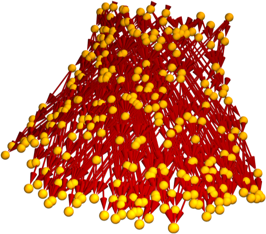
An example causal graph for a curved spacetime region.
The existence of this causal order is obviously compatible with special relativity, since as the only order that is observer independent is the order of causally related events. In fact, it has been shown that the causal order alone describes “9/10” of the structure of flat spacetime (Hawking et al 1976), as it fully describes the “shape”, but it is missing volume information. It is conjectured that this conclusion also holds for more general curved spacetimes described by General Relativity. In Causal Set Theory, this is known as the Benincasa-Dowker conjecture. In the context of the Wolfram Model, the emergence of General Relativity from causal graphs was described by Gorard (2020).
Entanglement Entropy on Causal Graphs
Entanglement Entropy on Causal Graphs
Like classical entropy, entanglement entropy measures information lost when performing a coarse graining of a system. In the case of entangled quantum systems, this happens when part of the entangled quantum system is not accessible. The full quantum state of a system can be described by a density matrix ρ. Performing a coarse graining is equivalent to taking the partial trace of the density matrix over the unobservable states, to obtain a reduced density matrix . The entanglement entropy can be calculated from the eigenvalues of the density matrix:
ρ
r
S=λlnλ
In Causal Set Theory, entanglement entropy is defined through a construction on scalar fields described by Sorkin (2012). Correlation functions can be obtained by computing Feynman propagators and Pauli-Jordan operators on the causal set, from these, a density matrix can be obtained and the entanglement entropy can be calculated.
This construction gives a covariant definition of entropy, as it is defined on an extended region of spacetime. This should not be surprising, as any calculation defined purely on the causal structure, which is observer independent, will yield observer independent results.
Gorard and Dannemann-Freitag (2023) provided on a Wolfram Language implementation of this procedure (see this post), which is available in the function repository as ResourceFunction[“CausalGraphEntanglementEntropyGeneralised”]. Once we obtain causal graphs compatible with a Schwarzschild geometry, we will employ this to calculate the entanglement entropy.
Methods
Methods
Our objective is to calculate the entanglement entropy of a Schwarzschild Black Hole. First, we will need to obtain a causal graph compatible with the Schwarzschild Geometry, next we will need to find a causal diamond lying on the interior of the Black Hole, from which we can then compute the entropy. By generating Black Hole causal graphs of different masses, and selecting causal diamonds of the same cardinality, we can test whether the
Generating the Causal graph
Generating the Causal graph
To obtain the causal graph for a Schwarzschild Black Hole, we start by decomposing the geometry in spacelike hypersurfaces. Since our objective is to calculate the entanglement entropy between the interior and the exterior regions, we choose a coordinate system that is regular at the horizon (it has no coordinate singularity). Our code can handle both Gullstrand-Painlevé and Eddington-Finkelstein coordinates, but we found it easier to obtain large causal diamonds using the former.
In[]:=
metric=ResourceFunction["MetricTensor"][{"IngoingGullstrandPainleve",1},{t,r,θ,ϕ}];metric["LineElement"]//TraditionalForm
Out[]//TraditionalForm=
2
d.s.
2
d.r
2
d.rd.t1
r
2
d.θ
2
r
2
d.ϕ
2
r
2
sin
2
d.t
2
r
The line element for ingoing Gullstrand-Painlevé coordinates. These are the coordinates of an infalling observer that started at zero velocity far away from the Black Hole.
In[]:=
decomposition=ResourceFunction["DiscreteHypersurfaceDecomposition"][metric,{t,0,1},{r,0,4},{θ,-Pi,Pi},200,1.5];hypersurfaceList=decomposition[{"CoordinatizedPolarGraphEvolutionColored",5}]
Out[]=
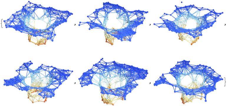
Decomposition in 6 spacelike hypersurfaces of the region t ∈ [0, 1], r ∈ [0, 4] with ϕ coordinate suppressed. The vertical coordinate and the color represent curvature.
We note that the hole in the graphs obtained here is not the location of the horizon, but the point at which excises the graph as the curvature became too large.
Next, we want to compute the causal relations between events from consecutive hypersurfaces. To do this, we extract the Cartesian vertex coordinates from the graphs above, convert them to polar coordinates, and add their time coordinate. Then for each pair of events we check whether their spacetime distance is timelike (i.e. negative), if so, we add an edge connecting the two. Once the full graph has been generated, we take the largest connected component to obtain a fully connected causal graph. The graph obtained in this way will be the transitive reduction of the full causal graph, which can be obtained by taking the TransitiveClosureGraph.
It is important to note that we can do this only because we choose a small time separation between hypersurfaces, and compute the distance between events that have a small coordinate separation. In general, the problem of determining causal connections is more complicated and requires integration of null geodesics to find the light cone.
In[]:=
generator=BlackHoleCausalSetGenerator[{"IngoingGullstrandPainleve",1},{40,10},{300,4}];causalGraph=generator["MakeCausalGraphCoordinatised"]
Out[]=
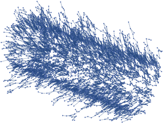
Causal graph for a Schwarzschild Black Hole
It is good to check that there are no connections escaping the interior, by highlighting the location of the horizon.
In[]:=
generator["HighlightedInteriorCoordinatised"]
Out[]=
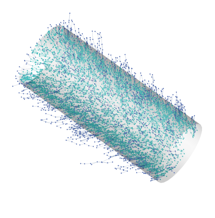
Interior region highlighted on a Schwarzschild causal graph. The cylinder represents the event horizon at a radius r = 2M.
Causal Diamonds
Causal Diamonds
The function ResourceFunction[“CausalGraphEntanglementEntropyGeneralised”] calculates the entanglement entropy between a causal diamond and a background causal set. Causal diamonds are patches of spacetime defined by the intersection of the causal future of an event and the causal past of another.
When doing so, it is important to be careful about edge effects: if the causal diamond includes vertices on the boundary of the background causal graph, the calculation will most likely fail. For this reason, we select a subgraph of the original graph before looking for causal diamonds.
Example of forwards and backwards light cones, highlighted in blue.
Causal graph with causal diamond highlighted in blue.
From here, we can easily compute the entropy:
Next, we need to locate a causal diamond in the interior region of the Black Hole. This proved challenging as without a large spatial resolution in our decomposition, there are not many large causal diamonds. This is because the light cones on the interior all bend towards the singularity, leaving very few causal connections between points in the region just behind the horizon.
ResourceFunction[“DiscreteHypersurfaceDecomposition”] can only discretize up to a certain point inside the Black Hole, after which the curvature becomes too large and the region is excised.
To find a large causal diamond we used a double optimisation approach: we first selected the ones that span the most along the time coordinate, which is very fast since it only accounts for the time difference between the start and the end point, and then among a list of longest causal diamonds we select the ones with the largest number of vertices, so as to make sure to get a causal diamond with some structure, instead of a single long chain of events.
Largest causal diamond in the interior region for the causal graph generated above.
Concluding remarks
Concluding remarks
Our current approach to determining the causal graph is limited to static and spherically symmetric metrics. Possible extensions include developing a generalised algorithm to compute causal relations by integrating null geodesics, which would allow to construct causal graphs for arbitrary curved spacetimes. Another limitation of our code is that it currently cannot handle very large graphs, making it hard to find good causal diamonds to compute the entropy.
Our code can be easily extended to 3+1 dimensions with minor tweaks, but it will likely be limited by computational constraints.
Keywords
Keywords
◼
Black Hole Entropy
◼
Entanglement Entropy
◼
Causal Graph
◼
Discrete Spacetime
Acknowledgment
Acknowledgment
I would like to thank my mentor, Jonathan Gorard, for his guidance and support throughout these four weeks. I also want to thank Mark Greenberg and Robert Nachbar for stepping in with help when I needed it, and Xerxes Arsiwalla for sparking some thought-provoking conversations. Lastly, all the staff and fellow participants of WSS 2023, who made this a highly educational and memorable experience.
References
References
◼
Bekenstein, J.D. (1973) ‘Black Holes and Entropy’, Physical Review D, 7(8), pp. 2333–2346. Available at: https://doi.org/10.1103/PhysRevD.7.2333.
◼
Bombelli, L. et al. (1987) ‘Space-time as a causal set’, Physical Review Letters, 59(5), pp. 521–524. Available at: https://doi.org/10.1103/PhysRevLett.59.521.
◼
Dannemann-Freitag, J., [WSS23] Looking at Network Packet Data with Wolfram Language and GPT Models - Online Technical Discussion Groups—Wolfram Community. [online] Available at: https://community.wolfram.com/groups/-/m/t/2956860 [Last Accessed 12 Jul. 2023].
◼
Gorard, J. (2021) ‘Algorithmic Causal Sets and the Wolfram Model’.
◼
Hawking, S.W., King, A.R. and McCarthy, P.J. (1976) ‘A new topology for curved space–time which incorporates the causal, differential, and conformal structures’, Journal of Mathematical Physics, 17, pp. 174–181. Available at: https://doi.org/10.1063/1.522874.
◼
Gorard, J. and Dannemann-Freitag, J. (2023). Axiomatic Quantum Field Theory in Discrete Spacetime via Multiway Causal Structure: The Case of Entanglement Entropies.
◼
Gorard, J . (2020) 'Some Relativistic and Gravitational Properties of the Wolfram Model', Complex Systems, 29 (2), pp. 599–654. Available at: https://doi.org/10.25088/ComplexSystems.29.2.599
◼
Sorkin, R.D. (2012) ‘Expressing entropy globally in terms of (4D) field-correlations’. arXiv. Available at: https://doi.org/10.48550/arXiv.1205.2953.
CITE THIS NOTEBOOK
CITE THIS NOTEBOOK
Black hole entanglement entropy from causal graphs
by Jacopo Uggeri
Wolfram Community, STAFF PICKS, July 12, 2023
https://community.wolfram.com/groups/-/m/t/2959318
by Jacopo Uggeri
Wolfram Community, STAFF PICKS, July 12, 2023
https://community.wolfram.com/groups/-/m/t/2959318