Abstract: We present a method to model the propagation of a transversal EM wave, which corresponds to a classical photon, through variable- dimensional space discretized on a graph. In particular, we show that the intensity of the wave gets amplified or damped, depending on the dimensional change which is in perfect agreement with recent results in the continuum [8]. The method used to achieve this result is to discretize the continuous solution which is obtained by solving the wave equation in variable-dimensional space. Furthermore, we present two more ansatzes which will be the matter of further investigation in the future: The fractional Laplacian Matrix and curvature as a model for fractional dimensional space (Appendix A and B). It turns out that, leaving boundary effects aside, curvature of discrete space mimics dimension change as the results are consistent with theoretical predictions in [8].
Contents
1. Introduction2. Wave equation on graphs 2.1 Method 1: Integer dimensional Laplacian Matrix 2.2 Method 2: Discretizing the continuum3. Heterodimensional graphs 3.1 Intrinsically fractional graphs 3.2 Extrinsically fractional graphs 3.3 Curvature as dimension change4. Method 2: Fractional dimensional solution on graphs5. Conclusions & Future Work 5.1 Conclusions 5.2 Laplacian Matrix in fractional dimensions 5.3 MiscellaneousAppendix A: Method 1: Laplacian MatrixAppendix B: Curvature as a model for fractional dimensions
1. Introduction
1. Introduction
Non integer dimensionality of space is in agreement with general relativity and could potentially solve current issues such as the anomalous magnetic moment of the electron [1,2,4]. In electromagnetic theory, the concept of fractional dimensionality of space-time allows to eliminate the
logarithmic divergence of quantum electrodynamics [5]. Furthermore, changes in dimensions such as from 2D to 1D appear all throughout physics such as in semiconductors and in MOSFETs to name just a few applications.
It is therefore of great interest to investigate wave propagation through variable-dimensional space, in particular through space of fractional dimensionality.
2. Wave equation on graphs
2. Wave equation on graphs
In essence there are two ways how the propagation of a photon, which boils down to the solution of a wave equation, can be implemented on a graph.
The first method uses the Laplacian Matrix [3,6] and will be described in the following subsection 2.2.1. It is well established in integer dimensions.
The second method which allows us to study wave propagation on a graph is to discretize the solution of continuous space and sample it on the vertices of the graph.
The advantage of the second method is that we can make use of the solid framework for fractional dimensions in continuous space and transfer it to discrete space modeled by graphs.
2.1 Integer dimensional Laplacian Matrix
2.1 Integer dimensional Laplacian Matrix
Let us start with the first way to realize wave propagation on graphs, which is via the Laplacian Matrix, also called the graph Laplacian or Kirchhoff Matrix. Given a simple graph G with a set of n vertices, the elements of the Laplacian matrix L are defined by

where deg stands for the degree of the respective vertex. This is a well-defined object on a graph, but so far efforts to capture fractional dimensionality of the operator have been rather rare, recent and most importantly quite tedious and technical [7]. This is why when we choose the approach of the Laplacian Matrix to describe the photon propagation, we impose the fractional dimensionality on the graph itself (see section 3.1). In other words, since the Laplacian Matrix is a priori defined for integer dimensions, the nature of fractional dimensionality needs to be captured by the structure of the graph and not by the operator. A preliminary, naive expectation is that this approach does not fully capture all effects of fractional dimensionality as one would expect also the operator to change in non integer dimensions when compared to integer dimensional space. Thus, one is naturally lead to investigate a definition of a Laplacian Matrix on a graph in fractional dimensions (see section 5.2 for an outlook).
The second important feature of this approach, besides the fact that the dimensionality is carried by the graph instead of the operator, is that, in analogy to dimensionality, also the initial conditions are inherent to the graph and not to the analytic solution of the equation. Said differently, the initial conditions of the wave equation need to be imposed on the graph by assigning the appropriate initial vertex weights since the method of the Laplacian Matrix only involves acting locally with the operator at each vertex of the graph, irrespective of the vertex weights and initial conditions.
To put it in a nutshell, the method of applying the Laplacian Matrix on a graph in order to describe the wave function naturally leads us to enforce the dimensionality and the initial conditions on the graph instead of the operator. Note that his stands in contrast to the second method of discretizing fractional dimensional solutions as described in section 2.2, where the operator as well as the analytic solution of the wave equation carry all relevant information and are subsequently discretized.
Let us now implement the wave equation and observe its propagation on the graph as described by the graph Laplacian (Laplacian Matrix) in integer dimensions.
In order to achieve this we follow the standard procedure of calculating the eigenvalues and eigenfunctions of the Laplacian operator, followed by projecting the initial conditions on the onto the eigenspace, performing the temporal evolution in the eigenspace and finally projecting back onto the real space.
This implementation has most notably been achieved by Jon Lederman in the WSS2020 [3] where he investigated the diffusion equation on a graph. Since we are looking at the wave equation instead, we solely need to change the solutions from exponentially decaying solutions to oscillatory ones.
In the following code we choose standing waves for the only reason that the intensity in 2D drops like 1/distance^2 and therefore would make it hard to observe the propagation further than a few vertices. At the end of this section the amplitude decay is visualized as a side note.
Starting out with a simple gird graph:
In[]:=
simpleGridGraph=GridGraph[{16,16},VertexSizeLarge,ImageSize350]AnnotationValue[simpleGridGraph,VertexWeight];
Out[]=
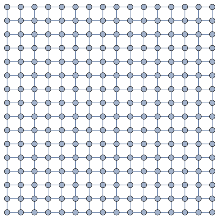
Figure 1: 16x16 Grid Graph
We can now define the necessary functions to assign vertex weights as amplitudes on a graph (in analogy to Jon Lederman’s temperatures):
In[]:=
(*Returnstheamplitudesonagraph*)Getamplitudes[g_]:=AnnotationValue[g,VertexWeight];(*TakesagraphandamplitudevaluesandsetsthevaluesonthegraphastheVertextWeight*)Attributes[Setamplitudes]={HoldFirst};Setamplitudes[g_,amplitudes_]:=AnnotationValue[g,VertexWeight]=amplitudes;(*Colorsagraphusingaamplitudelist*)ColorByamplitude[g_,amplitudes_]:=HighlightGraph[g,MapThread[Style,{VertexList[g],Map[ColorData["Rainbow"],amplitudes]}]];(*Colorsagraphbyitsinternalamplitudes(fromALREADYassignedVertexWeightsobtainedbyGetamplitudes)*)ColorByInternalamplitude[g_]:=ColorByamplitude[g,Getamplitudes[g]];
Let us choose the initial condition of a delta function in the center of the graph:
Let us choose the initial condition of a delta function in the center of the graph:
In[]:=
(*Setsadeltafunctiononagraphatvertexofsizedistanceforic*)SetDeltaFunction[g_,vertex_,distance_]:=Module[{ng=g},(AnnotationValue[{ng,#},VertexWeight]=ConstantArray[1,Length[#]])&@VertexList[NeighborhoodGraph[g,vertex,distance]];ng];
Finally, we use the code segments of Jon Lederman as described above which involves the time evolution in the eigenspace of the Laplacian:
Finally, we use the code segments of Jon Lederman as described above which involves the time evolution in the eigenspace of the Laplacian:
In[]:=
(*ThefollowingcodecalculatesthegraphLaplaciananditsspectrum.UnnormalizedLaplacianreturnstheunnormalizedLaplacianoftheassociatedundirectedgraph.AdjMatrixconvertsadirectedgraphtoanundirectedgraphandcalculatestheadjacencymatrix.GraphSpectrumreturnstheeigenvaluesandeigenfunctionsofthegraphinputobjectasanassociativearray.*)UnnormalizedLaplacian[g_]:=N@(DiagonalMatrix[VertexOutDegree[#]]-AdjacencyMatrix[#])&@UndirectedGraph[g];AdjMatrix[g_]:=N@AdjacencyMatrix[#]&@UndirectedGraph[g];GraphSpectrum[g_]:=<|"eigenvalues"Eigenvalues[#],"eigenvectors"Eigenvectors[#]|>&@UnnormalizedLaplacian[g];(*Thefollowingcodeimplementstheheatkerneldynamics.*)(*Projectinitialconditionsontoeigenspace*)EigenSpaceProject[ic_,eigenvectors_]:=eigenvectors.ic;(*Projectvector,whichmaybeatimeevolvedvectorineigenspaceontovertexspace(amplitudespace)*)VertexSpaceProject[vector_,eigenvectors_]:=Transpose[eigenvectors].vector;(*Performtemporalevolutionineigenspace*)(*Oscillatoryeigensolutions*)EigenSpaceAdvance[spectrum_,coordinates_,t_]:=(Cos[1/10*t*spectrum["eigenvalues"]]+Sin[1/10*t*spectrum["eigenvalues"]])*coordinates;(*Performtemporalevolutioninamplitude/vertexspace*)amplitudeSpaceAdvance[spectrum_,ic_,t_]:=VertexSpaceProject[EigenSpaceAdvance[spectrum,EigenSpaceProject[ic,#],t],#]&@spectrum["eigenvectors"];(*Thefollowingfunctiontemporallyadvancestheheatdistributiononagraphbymodifyingtheprovidedgraphobject*)Attributes[TimePropagate]={HoldFirst};TimePropagate[g_,t_]:=Setamplitudes[g,amplitudeSpaceAdvance[GraphSpectrum[g],Getamplitudes[g],t]];
Note that in the function EigenSpaceAdvance we have inserted oscillatory solutions.
To wrap up this section, we want to see some animations of how the wave actually propagates:
Note that in the function EigenSpaceAdvance we have inserted oscillatory solutions.
To wrap up this section, we want to see some animations of how the wave actually propagates:
In[]:=
(*Startwithemptygrid*)Setamplitudes[simpleGridGraph,ConstantArray[0,256]];ColorByInternalamplitude[simpleGridGraph];(*Initialcondition:Deltafunctioninthegraphcenter*)deltaGridGraph=SetDeltaFunction[simpleGridGraph,First[GraphCenter[simpleGridGraph]],1];ColorByInternalamplitude[deltaGridGraph];(*Generatelistofimagesforanimation2D*)animation2DTable=Table[TimePropagate[deltaGridGraph,t];ColorByInternalamplitude[deltaGridGraph],{t,Table[i,{i,1,10,0.5}]}];ListAnimate[animation2DTable]
Out[]=
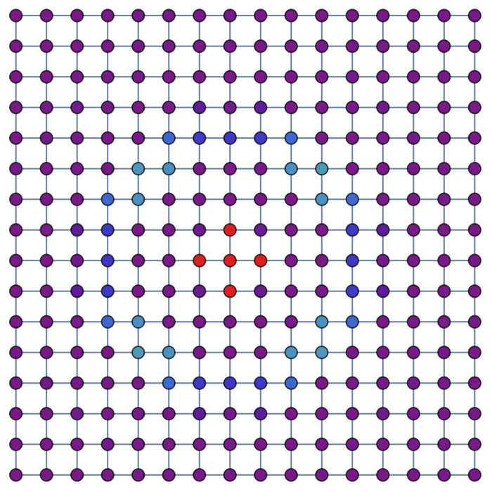
Figure 2: Spherical wave propagation with the graph Laplacian method on a 16x16 Grid Graph.
And indeed we see some neatly outwards propagating, spherical waves!
2.2 Discretizing the continuum
The other method to describe wave propagation on a graph involves finding the solution to the wave equation and discretizing it on the graph.
For homogenous ODEs one obtains a homogenous solution, whereas for inhomogeneous ODEs one must find the Green’s function of the wave equation first.
The Green’s function describes the response to a point source in time and space. The total solution can be obtained by superposition of the partial solutions and uniqueness is guaranteed by imposing a set of appropriate initial conditions on the system.
Since this method yields the most consistent results in capturing fractional dimensionality, we dedicate an entire section (section 4) to it where the steps and solutions are presented in detail.
For the moment, it suffices that the reader is aware of the fact that this method exists and is expected to produce relevant results.
3. Heterodimensional graphs
3. Heterodimensional graphs
2D Face docking
Now create an analogous function as above, but this time just for merging the 2D region with the 3D region at a face of the cube instead of at the corner.
Now create an analogous function as above, but this time just for merging the 2D region with the 3D region at a face of the cube instead of at the corner.
Now, create the final function that adds a new graph of lower Hausdorff dimension to the 3D graph:
Before moving on to fractional dimensions, here are two neat examples for corner and face merging respectively:
Example for Corner Merging & Face Merging
Figure 3 & 4: Examples for merging 2D and 3D graphs. Left: Example for corner merging between a 3D cube graph and a 2D planar grid graph. Right: Face merging between the same graphs.
To conclude, this approach of “graph surgery” allows us to chain graphs of arbitrary dimensions and shapes together. That is to say, it opens up the possibility to create heterodimensional graphs (graphs with regions of different dimensions).
Now that we are equipped with the necessary tools to chain regions of different dimensions together, let us look at fractional dimensionality of graphs.
Now that we are equipped with the necessary tools to chain regions of different dimensions together, let us look at fractional dimensionality of graphs.
3.1 Intrinsically fractional graphs
For the ansatz using the Laplacian Matrix we need the graph itself to have regions of inherently different dimensions simply because the Laplacian Matrix is an object that does not depend on the local dimension of the graph itself. Thus, one way to solve this issue is to rely on graphs that have an intrinsic fractional dimension, such as the Sierpiński graph. The Sierpiński graph is an example for a fractional dimensional graph with a Hausdorff dimension that converges to log(3)/log(2) ≈ 1.585.
To capture the entire effect of the noninteger dimensionality, a wave front (for which the wave length is an appropriate measure) should be much larger than one Sierpiński triangle.
In other words, the wavelength should include as many Sierpiński triangles as possible. The following image shows a Sierpiński graph in 3D with three subtriangles:
Figure 5: Example for a Sierpiński graph in 3 dimensions.
Finally, let us chain together some integer dimensional region with a Sierpiński graph for demonstration purposes:
Figure 6: The “fish graph” - Example for merging a Sierpiński graph with a 2D grid graph.
3.2 Extrinsically fractional graphs
Figure 7: Extrinsic insertion of dimension perturbation. The region with a fractional dimension is highlighted by larger vertex sizes.
The fractional dimensional solution of the wave equation, which is an explicit function of the dimension, can then assign different (fractional) dimensions to the different graph regions.
The fractional dimensional solution of the wave equation, which is an explicit function of the dimension, can then assign different (fractional) dimensions to the different graph regions.
3.3 Curvature as dimension change
A third way to model a change in dimension of a graph, in particular to reach a fractional dimension, is to introduce curvature to a graph with integer Hausdorff dimension.This can be done by inserting new edges between nonadjacent vertices.
This way of mimicking dimension change can be seen as another option for introducing intrinsically fractional dimensions since the graph and its structure are modified, contrary to the extrinsic method in 3.2 where the dimension is only assigned and the shape of the graph remains unchanged.
We would expect that a propagating EM wave on a graph with appropriate curvature should then reproduce the results from extrinsic dimension assignment as in 3.2.
We will see in Appendix B.2 that this is indeed the case and that the results are consistent.
4. Fractional dimensional solution on graphs
4. Fractional dimensional solution on graphs
The overarching goal is to describe the propagation of a photon trough fractional dimensional space and/or regions of varying dimensions.
In this section we will solve this problem with the method of discretizing the continuous solution.
In continuous space, the Laplacian for non integer dimensions in spherical coordinates is given by [9]
In this section we will solve this problem with the method of discretizing the continuous solution.
In continuous space, the Laplacian for non integer dimensions in spherical coordinates is given by [9]
where D is the dimension. In cylindric coordinates it is given by [8,10]
The homogenous (or source free) wave equation then takes the well-known form
Note the dependency on the dimensionality in the field as well as in the spatial derivative operator.
As long as we look at 2D grid graphs we stick to the cylindric form of the Laplacian. In the following, we will investigate the setting of 2D grid graphs with a light flash (electromagnetic field) originating in the graph center as this specific setup allows us to make use of some simplifications and provides a clean analytic solution. In particular, the z-component can be disregarded as we are working on a plane. Furthermore, there is no well defined azimuthal angle on a graph and, nevertheless, we work in azimuthal symmetry due to the spherical shape of the light flash. Thus, the only relevant part of the equation is the radial one and after separation of variables one obtains the solution [8]
Figure 8: The amplitude of the EM wave in fractional dimension 1.585 < 2(blue) and in integer dimensions (orange). Note that the fractional dimension here corresponds to the Hausdorff dimension of the Sierpiński graph.
Figure 9: The amplitude of the EM wave in fractional dimension 2.3 > 2 (blue) and in integer dimensions (orange).
Thus, we see a damping / amplifying effect of fractional dimensions on EM waves which is in accordance with [8] (see e.g. figures 2, 3 and 4 in their article).
Finally, let us discretize this behaviour and investigate it on a graph. As described in the previous sections, for the analysis of light propagation through variable dimensions in a graph we choose the second method, i.e. discretizing the solution to the wave equation.
The following code contains the implementation of this solution as a function of space (discrete variable), time (continuous variable) and the dimension (continuous variable):
For the sake of simplicity, let us start with integer dimensions.
Visualizing the wave with some appropriate initial conditions on a 2D grid graph (integer dimension) yields:
For the sake of simplicity, let us start with integer dimensions.
Visualizing the wave with some appropriate initial conditions on a 2D grid graph (integer dimension) yields:
Figure 10: Solution to the fractional dimensional wave equation in the special case of integer dimension.
As expected, we see neat oscillations in space with a radially decaying amplitude.
A more delicate feature of this method is that, contrary to the Laplacian matrix, the metric of the space is respected. In particular, while in Figure 2 the propagation is spherical even though the wave propagates in a grid graph, for the discretization method the wave is square shaped which corresponds to a “sphere” on a grid. Therefore, the shape of the wave matches with the respective internal graph structure, which is ensured by the function GraphDistance that is not present in the Laplacian Matrix method.
Of course we also want to look at fractional dimensions:
Example for perturbed space (see previous section) we can choose the fractional dimension to be 1.585 and obtain the following animation.
Example for perturbed space (see previous section) we can choose the fractional dimension to be 1.585 and obtain the following animation.
Figure 11: Wave amplification in fractional dimension 1.585 < 2.
As we can see, there is a perturbed region in the 2D graph, visualized by larger vertex sizes. The dimension of the perturbed region is 1.585 < 2.
From the color coding it is clearly visible that the amplitude in this region is amplified which is in perfect agreement with the continuum case calculated by [8].
From the color coding it is clearly visible that the amplitude in this region is amplified which is in perfect agreement with the continuum case calculated by [8].
On the contrary, we can also look at a perturbation in a higher fractional dimension where we would expect the amplitude to be damped.
For example, let us look at the graph above but this time with a localized region of increased fractional dimension d = 2.4 > 2.
For example, let us look at the graph above but this time with a localized region of increased fractional dimension d = 2.4 > 2.
Figure 12: Wave damping in fractional dimension 2.4 > 2.
In agreement with [8] in the continuum we see the damping of the amplitude when the fractional dimension lies above the integer dimension.
5. Conclusion & Future Work
5. Conclusion & Future Work
5.1 Conclusion
We have seen that when choosing the sampling method, i.e. discretizing the continuous solutions to the wave equation, one observes amplification or damping of the intensity in regions of fractional dimensions.
This result is in agreement with previous results [8,9] and appears to hold true on graphs in the scope of EM waves with cylindric symmetry.
We saw that we can choose an arbitrary fractional dimension and draw conclusion on its amplification / damping effect on an EM wave traveling through this fractal medium.
5.2 Future Work
Further work based on this project would be to generalize the Laplacian Matrix (Method 1) on graphs for fractional dimensions to see if the results are consistent with the discretization method.
To test the fractional Laplacian Matrices, the matrix can be acted upon an intrinsically fractional dimensional graph. These intrinsic fractional dimensional structures can be implemented in a straight forward manner using tools presented in section 3 in order to create intrinsic heterodimensional graphs. The Resource Function GraphMerge is available on the Wolfram Function Repository and combines all the functionalities demonstrated in section 3.
Another line of investigation that opened up is to look at inhomogeneous wave equations, i.e. when there is a source present. This has been treated analytically in the continuum by [9] (see chapter 18 therein).
Finally, one can also explore the concept of curvature and how this can model non integer spatial dimensions. The foundation for this is presented in Appendix B.
5.3 Miscellaneous
- Submission of Resource function for creating heterodimensional graphs
- Submission of Resource function that visualizes arbitrary wave equations
- Submission of Resource function for creating grid graphs with crossbars
- Submission of Resource function that visualizes arbitrary wave equations
- Submission of Resource function for creating grid graphs with crossbars
Keywords
Keywords
◼
Fractional dimensions
◼
Photon propagation
◼
Wave equation
Acknowledgment
Acknowledgment
I want to thank Stephen Wolfram for defining this extremely exciting project, for his initial ideas as well as for his constructive feedback.
I want to thank Jon Lederman and Tom Lee for the excellent supervision they have provided and their encouragement throughout the entire process.
Furthermore, I want to thank Jonathan Gorard for fruitful discussions, and also Hans Christiansen for productive the exchange of ideas.
Finally, I want to thank every mentor, participant and organizer of this amazing Summer School. It was truly one of the most unique and best research experiences that I had so far.
Appendix A: Method 1: Laplacian Matrix
Appendix A: Method 1: Laplacian Matrix
In section 2.1 we have discussed the method of applying the Laplacian Matrix to the graph as a way to implement wave propagation on graphs. At least in integer dimensions this yields consistent results.
However, when turning towards fractional dimensional graph sections, there is no change in intensity observable which disagrees with the results from the discretization method as well as with the results for continuous space.
Therefore, the expectation is that the Laplacian Matrix in its form from 2.1 cannot fully capture a fractional dimension, even less a change in dimensionality in the first place.
The conclusion from this is that one would need to generalize the current concept of a Laplacian Matrix to fractional dimensions which is part of the future work resulting from this project.
In order to illustrate the flaw in this approach, the code segment below shows the propagation of a wave with an initial delta function originating in a 2D region and spreading into a 1.585 dimensional region.
It is clearly visible that there is no change in amplitude, nor do any other visible differences appear.
Note that for computational efficiency the graph has been drastically reduced in size which implies that boundary effects become relevant relatively quickly.
Figure A.1: Propagation with Laplacian Matrix method on a Grid Graph (2D) transitioning to Sierpinski graphs (intrinsic dimension of 1.585).
At least heuristically we do not see a change in intensity in the first maximum when compared to the animation shown on a 2D plane in section 2.1.
This leads to the conclusion that indeed the operator (i.e. Laplacian Matrix) needs to change in a fractional dimension to fully capture its effect.
This leads to the conclusion that indeed the operator (i.e. Laplacian Matrix) needs to change in a fractional dimension to fully capture its effect.
Appendix B: Curvature as a model for fractional dimensions
Appendix B: Curvature as a model for fractional dimensions
Curvature on a grid graph, which is implemented by adding new edges, results in a different Hausdorff dimension when compared to the regular 2D case.
We will use method 1 (i.e. the Laplacian Matrix) in this subsection. For the use of method 2 see the next section B.2.
For the purpose of illustration and simplicity let us begin with an very localized perturbation in curvature on a 2D grid graph.
We will use method 1 (i.e. the Laplacian Matrix) in this subsection. For the use of method 2 see the next section B.2.
For the purpose of illustration and simplicity let us begin with an very localized perturbation in curvature on a 2D grid graph.
Figure Figure B.1.1: Wave propagation with Laplacian Matrix method on a grid with local perturbation.
We see that the propagation of the wave in the vicinity of the perturbation will have progressed further than far away from the perturbation.
This agrees with the intuitive expectation that a reduction in distance (which is what we effectively do when adding new edges) leads to a faster propagation.
This agrees with the intuitive expectation that a reduction in distance (which is what we effectively do when adding new edges) leads to a faster propagation.
To wrap up this section, let us look at a graph that looks more like an interface between media to get a better intuition for curvature on a grid graph.
Figure B.1.2: Wave propagation with Laplacian Matrix method on a grid with an interface between regions of different Hausdorff dimensions.
Again, qualitatively, we see a wave that appears to propagate faster.
However, it remains matter of investigation if this really corresponds to a change in propagation speed of the wave (which might be connected to a dimension change) or if it solely comes from the reduction of the distance in the spatial regions of fractional dimension.
However, it remains matter of investigation if this really corresponds to a change in propagation speed of the wave (which might be connected to a dimension change) or if it solely comes from the reduction of the distance in the spatial regions of fractional dimension.
Analogous to section B.1 we can also investigate the curvature as a potential model for fractional dimensions with the second method (discretization).
In this case, we estimate the dimension which appears explicitly in the potential by the Hausdorff dimension.
Boundary effects are clearly visible as the estimation of the Hausdorff dimension is local and only in the limit of an infinitely large grid one obtains exact values.
Nevertheless, the amplification of the amplitude is clearly visible, which suggests that for future work this may be an interesting path to follow as curvature of space appears to correctly reflect a change in dimensions.
(The animation can be seen below - the code is beneath the animation due to long run time ~ 4 minutes)
Code for the animation above (Attention: Run time ~ 4 minutes due to local Hausdorff estimation at each vertex at each time step):
References
References
◼ [1] Zeilinger A, Svozil K (1985) Measuring the dimension of space-time. Phys Rev Lett 54:2553–2555
◼ [2] Stillinger FH (1977) Axiomatic basis for spaces with noninteger dimension. J Math Phys 18:1224–1234
◼ [3] Jon Lederman: “[WSS20] Weyl’s law and The Wolfram Model of physics”
◼ [4] He X (1990) Anisotropy and isotropy: a model of fraction-dimensional space. Solid StateCommun 75:111–114
◼ [5] Matos-Abiague A (2001) Bose-like oscillator in fractional-dimensional space. J Phys A Math Gen 34: 3125–3128
◼ [6] Fan Chung: “SPECTRAL GRAPH THEORY” (1997)
◼ [7] Lidia Aceto et al.: “Fractional Laplace operator in two dimensions, approximating matrices, and related spectral analysis” (2020)
◼ [8] M. Zubair and M. J. Mughal: “An Exact Solution of the Cylindrical Wave Equation for Electromagnetic Field in Fractional Dimensional Space”
◼ [9] Dumitru Baleanu • Jose Antonio Tenreiro Machado, Albert C. J. Luo: “Fractional Dynamics and Control” - Chapter 18 by Sami I. Muslih and Om P. Agrawal
◼ [10] Schoener, Kyle and Varieschi, Gabriele: “Laplace’s Equation in Fractional-Dimension Spaces” (2021). Honors Thesis. 392.
CITE THIS NOTEBOOK
CITE THIS NOTEBOOK
Photon propagation through variable-dimensional space
by Simon Fischer
Wolfram Community, STAFF PICKS, July 19, 2022
https://community.wolfram.com/groups/-/m/t/2574806
by Simon Fischer
Wolfram Community, STAFF PICKS, July 19, 2022
https://community.wolfram.com/groups/-/m/t/2574806