Pharmacokinetic modeling uses differential equations to predict how drug concentrations change over time. These models play an important role in optimizing dosing regimens, especially for drugs with small therapeutic ranges. This project investigates the use of pharmacokinetic compartment models to simulate and optimize dosing regimens, with glibenclamide, a drug used to treat type 2 diabetes. One compartment, two compartment, and transit compartment models were developed and implemented using systems of ordinary differential equations. Analytical solutions were used to evaluate drug concentrations relative to therapeutic thresholds. Drug-specific pharmacokinetic parameters for glibenclamide were then incorporated into the models to simulate realistic drug amount–time plots and investigate the effects of varying dose size, dosing interval, and elimination rate. The results demonstrate that increasing model complexity and considering patient to patient variations provide more physiologically realistic predictions of oral drug absorption. The optimized dosing regimen maintained concentrations within the therapeutic range.
Introduction
Introduction
Pharmacokinetics
Pharmacokinetics
In pharmacokinetics (PK), differential equations are used to model plasma drug concentrations over time after each dose. Compartment models predict the rate at which a drug moves from one compartment to the next through the four stages of ADME: absorption, distribution, metabolism, and excretion. Through pharmacokinetic modeling, continuous prediction of drug concentration can be done in the bloodstream to develop the optimal dosing regimens in order to keep the drug amount in the desired therapeutic range. This modeling is crucial for drugs with a smaller therapeutic range, meaning when the drug amount is too low it becomes ineffective and when it is too high it becomes toxic. Carefully optimizing dosing regimens to stay in the desired therapeutic interval is crucial for ensuring the drug is safe and effective.
These models apply first-order kinetics where a percentage of drug moves per unit of time. In a one compartment model, the drug enters the bloodstream instantaneously and models IV infusion dosing. The drug is expected to rapidly distribute throughout the body. In contrast, a two compartment model separate the body into a absorption compartment (the stomach) and a central compartment (the bloodstream). As a result, the drug amount-time curve has two distinct phases: an initial distribution phase with a steeper slope as the drug rapidly spreads into peripheral tissue from the bloodstream and a slower elimination phase where the drug is being removed from the body (Robinson, 2025). This is characterized by a flatter slope.
However, many oral medication have a significant delay between administration and absorption into the bloodstream due to processes like gastrointestinal movement (Bashiardes & Christodoulou, 2024). To better represent this delay, transit compartment models can be used to split the absorption process into steps to more accurately model the delayed absorption. In these models, the drug moves through the transit compartments at a constant transit rate before reaching the central compartment. The number of transit compartments and the transit rate determine the time it takes the drug to reach the bloodstream. This represents the drugs with slower absorption more strongly in order to improve plasma drug level predictions and identify more efficient dosing regimens that stay within the therapeutic range.
Type 2 Diabetes Glibenclamide Drug
Type 2 Diabetes Glibenclamide Drug
In the U.S., 1 in 10 individuals has diabetes and about 90 to 95 percent of them develop Type 2 diabetes mellitus (T2D) (Cleveland Clinic, 2025). When a patient has T2D, their body can not use insulin properly leading to blood glucose build up and hyperglycemia. If left untreated, hyperglycemia can cause cardiovascular disease, nerve damage, kidney damage, and damage to the blood vessels in the retina leading to blindness (Mayo Foundation for Medical Education and Research). It is important to treat T2D to avoid these complications and to better patient lives.
Glibenclamide is one common treatment for T2D. Glibenclamide is an oral medication that promotes the release of insulin from pancreatic beta cells to reduce blood glucose in the body (Rambiritch et al., 2014). This increase in insulin helps lower blood glucose levels returning to glucose homeostasis. However, because glibenclamide has a small therapeutic range, maintaining drug levels between the upper and lower therapeutic thresholds is important. When plasma drug level is too low, it results in inadequate glucose control, and when it is too high, it can lead to hypoglycemia.
To find an optimal dosing regimen for glibenclamide, it is crucial to model how drug concentrations change over time in the body with different dosing regimens and patients. PK modeling can use differential equations to explain these drug concentration changes and predict the effects of different dosing regimens. By using compartment models, such as one-compartment, two-compartment, and transit compartment models, drug behavior can be simulated to optimize dosing regimens and improving personalized treatments for Type 2 diabetes patients.
Glibenclamide dosing regimens are limited because a greater dose doesn’t result in more therapeutic benefit. In a 12-week dose-escalation study, Rambiritch et al. found that increasing the daily dose from 2.5 mg to 20 mg resulted in no significant additional reduction in blood glucose or increase in insulin secretion compared to the 2.5 mg dose. There are also patient to patient differences in pharmacokinetic characteristics, such as drug absorption, metabolism, and elimination, so fixed dosing regimens may not work for every patient. These limitations highlight the need for drug course over time modeling and personalized dosing regimens, especially for glibenclamide (Rambiritch et al., 2014).
Objectives
Objectives
1. Demonstrate pharmacokinetic compartment models to simulate drug dosing regimens including bolus dosing and loading doses from the Hof and Bridge paper.
2. Analyze how pharmacokinetic parameters and dosing regimens effect drug levels over time.
3. Demonstrate how pharmacokinetic modeling can optimize glibenclamide dosing regimens by identifying regimens personalized to individual patients that maintain desired therapeutic levels.
Model Setup
Model Setup
Input Equations/Dosing Regimen
Input Equations/Dosing Regimen
In a 2020 methodological study, Hof and Bridge developed an ordinary differential equations (ODE) system with analytical solutions for drug amount over time for three different compartment models. These models used forcing equations to represent drug input to allow modeling different dosing regimens and administration methods. The forcing equations explain how the drug enters the compartment system over time to simulate changes in drug amount in the bloodstream.
The Equi-bolus regimen (Beq) is a dosing strategy where the same amount of drug is given as a bolus dose (administered rapidly as a single dose). In this regimen, M identical doses of size D0 are given at evenly spaced intervals T. The Dirac Delta function is used to represent these instantaneous drug doses at specific points in time.
Function gB models the input rate which considers bioavaliability, dose, and time interval:
In[]:=
gB[t_]:=Sum[F*D0*DiracDelta[t-(j-1)T],{j,1,M}]
The Equi-bolus regimen with a loading dose (BeqL) is a dosing strategy where a loading dose (a larger first dose used to quickly reach the desired drug amount) is given once before using the regular maintenance doses. The maintenance bolus doses D0 are given at evenly spaced time intervals T for M doses. The Dirac Delta function is used to represent these instantaneous drug doses.
Function gBL models the input rate which considers bioavaliability, dose, and time interval:
In[]:=
gBL[t_]:=F*DL*DiracDelta[t]+Sum[F*D0*DiracDelta[t-(j-1)T],{j,2,M}]
Parameters
Parameters
One-Compartment Model
One-Compartment Model
Compartment Model Diagram
Compartment Model Diagram
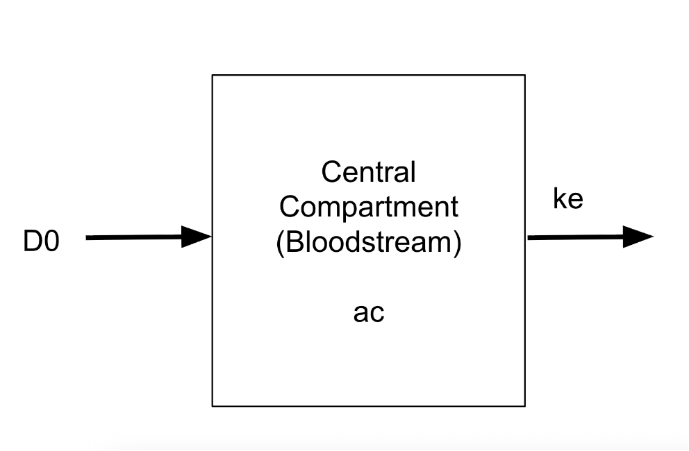
This is a diagrammatic representation of a one compartment model. An input dose (D0) directly enters the central compartment (bloodstream) and leaves at a rate of ke (first order process). This models drug infusion with ac representing the amount of drug in the central compartment. I made this diagram in Google Drawings.
Initial Value Problem Equations
Initial Value Problem Equations
Initial value problems (IVPs) are a math technique that uses differential equations with initial conditions provided to model how a system changes over time. In this case, the IVPs are applied to explain changes in drug levels by modeling movement, absorption, and elimination in the body. For a one-compartment model, the rate of change of drug amount in the bloodstream depends on the drug input rate from the dosing regimen and the elimination rate. Different IVP equations were collected for each dosing regimen to account for differences in drug administration. These equations below are collected from the Hof and Bridge study.
For the Beq regimen, the change in drug amount in the bloodstream is modeled using the input rate from the dosing equation gB(t) minus the elimination of the drug from the body:
In[]:=
solM1Beq=ac'[t]==-keac[t]+gB[t],ac[0]==0;
For the BeqL regimen, the change in drug amount in the bloodstream is modeled using the input rate from the dosing equation gBL(t) with a loading dose minus the elimination of the drug from the body:
In[]:=
solM1BeqL=ac'[t]==-keac[t]+gBL[t],ac[0]==0;
For the Ieq regimen, the change in drug amount in the bloodstream is modeled using the input rate from the dosing equation gI(t) minus the elimination of the drug from the body:
In[]:=
solM1Ieq=ac'[t]==-keac[t]+gI[t],ac[0]==0;
Derivation
Derivation
The Laplace transform was used to derive the analytical solution for the one compartment model for the Beq dosing regimen. The calculation began with the initial value problem from earlier. The input rate was represented with instantaneous doses using the Dirac delta function. The Laplace transform was used to change the differential equation into an algebraic equation that was easier to solve for the drug amount. The solution comprised of a summation of exponentially decaying piecewise functions from each dose. The Heaviside step function ensured that each dose only influenced the drug amount after it was given. This final analytical form was used to simulate drug amount over time with multiple doses.
This is the Beq regimen initial value problem from earlier:
In[]:=
′
ac
Here gB(t) is the equation used to model drug input. It uses Dirac Delta to show discrete drug doses:
gB(t)=FD0δ(t-(j-1)T)
M
∑
j=1
The Laplace transform of the initial value problem is taken:
In[]:=
′
ac
The Laplace transform is applied to both sides of the differential equation:
L((t))=GB(s)-keAc(s)
′
ac
Using the Laplace transform of a derivative, the initial condition appears:
L((t))=sAc(s)-Ac(0)=sAc(s)
′
ac
Since there is no drug in the compartment initially:
In[]:=
Ac(0)=0
The Laplace transform of whole equation:
In[]:=
sAc(s)=GB(s)-keAc(s)
Rearranging:
In[]:=
Ac(s)=
GB(s)
s-ke
The Laplace transform of the forcing function is evaluated using its integral definition:
In[]:=
GB(s)=L(gB(t))=FD0δ(t-(j-1)T)t
∞
∫
0
-st
e
M
∑
j=1
The summation is moved outside the integral:
In[]:=
L(gB(t))=FD0δ(t-(j-1)T)t
M
∑
j=1
∞
∫
0
-st
e
Applying the sifting property of the Dirac delta function:
In[]:=
GB(s)=FD0
M
∑
j=1
-(j-1)Ts
e
Substituting the transformed input function creates the complete solution:
In[]:=
Ac(s)=FD0
M
∑
j=1
-(j-1)Ts
e
s+ke
A substitution is used to simplify the inverse Laplace transform:
In[]:=
let(j-1)T=t0
The inverse Laplace transform:
In[]:=
InverseLaplaceTransform[Exp[-t0s]/(s+ke),s,t]
Out[]=
ke(-t+t0)
Heaviside Theta = H. This resulted in the analytical form:
In[]:=
ac(t)=FD0H(t-(j-1)T)
M
∑{
j=1
-ke(t-(j-1)T
e
Analytical Form for ac(t)
Analytical Form for ac(t)
The analytical form for ac(t) models the amount of drug in the bloodstream with repeated dosing.
The analytical form is represented in Wolfram Language:
In[]:=
ac[t_]:=F*D0*Sum[HeavisideTheta[t-(j-1)*T]*Exp[-ke*(t-(j-1)*T)],{j,1,M}]
where:
In[]:=
t-(j-1)T=tj=timesincejthdose
so:
In[]:=
ac(t)=FD0H(tj)
M
∑
j=1
-ke(tj)
e
Plotting Drug Time Course
Plotting Drug Time Course
The analytical form of ac(t) was used to model drug amount over time in the central compartment for the Beq regimen. The plot can be used to investigate how changes in pharmacokinetic parameters affect drug levels in the bloodstream. A Manipulate function was used to provide sliders to test various bioavailability (F), dose (D0), interval (T), elimination rate (ke), and number of doses (M) values and visualize the effect. This allows for the testing of different dosing regimens and exploring effects of variation in people’s absorption and elimination rates. This plot takes the range of parameter values explored for a hypothetical drug in the Hof and Bridge paper. This is a demonstration of how the model works.
The Plot function graphed ac(t) using the analytical solution from earlier. As the user moves the sliders, the time course automatically updates:
The analytical form of ac(t) was used to model drug amount over time in the central compartment for the Beq regimen. Instead of sliders, discrete values are provided for parameters including F, D0, T, ke, and M. These discrete values come from the parameters of the hypothetical drug used in the Hof and Bridge study. The plot can be used to test if the Hof and Bridge paper was appropriately replicated. A Manipulate function was used to provide discrete values to test the F, D0, T, ke, and M values of the drug and visualize its effect. This can easily be extended to other drugs. M doesn’t matter other than giving the drug time to reach its proper drug fluctuation state so various parameters were provided for this. Additionally, the shaded region represents the safe and effective therapeutic threshold bounded by the upper and lower threshold. The therapeutic range is presented for testing purposes. The values are not from the paper. Additionally, this graph has discontinuities because of the DiracDeltas and HeavisideThetas, which are inherently discontinuous, used to model a discontinuous process like taking injections or pills.
The analytical equation from earlier was used to plot drug course over time. A plot was created using Manipulate and Plot. The filling functionality along with the upper and lower bounds were used to create the therapeutic range on the plot:
Two-Compartment Model
Two-Compartment Model
Compartment Model Diagram
Compartment Model Diagram
This is a diagrammatic representation of a two compartment model. An input dose (D0) enters the absorption compartment (stomach) which transfers to the central compartment (bloodstream) with a rate of ka (first order process). The drug exits the bloodstream with a rate of ke (first order). ab is the amount of drug in the stomach and ac is the amount of drug in the bloodstream. I made this diagram in Google Drawings.
Initial Value Problem Equations
Initial Value Problem Equations
The two-compartment model includes an absorption compartment to model the absorption process before the drug reaches the bloodstream. The IVP equations explain how the drug enters the stomach, transfers to the bloodstream, and gets eliminated. The absorption compartment is affected by the drug input and ka, while the central compartment is affected by drug absorption and ke.
Change in drug level in bloodstream is modeled using the input rate (gB(t)) minus the elimination rate for the Beq regimen in the two compartment model.
Change in drug level in bloodstream is modeled using the input rate (gBL(t)) minus the elimination rate for the BeqL regimen in the two compartment model.
Derivation
Derivation
The two compartment model additionally includes an absorption compartment so the IVP is rewritten in matrix form and solved using the Laplace transform to find the analytical form of ac(t).
Beq regimen initial value problem from earlier for a two compartment model:
gB(t) is used to model drug input. It uses Dirac Delta to show discrete drug doses:
Rewrite model’s equations as a matrix:
Matrix differential equation:
Laplace transform:
Initial condition:
Rearranging:
Multiplies by the inverse matrix to solve for the solution:
Calculates the matrix sI − B
Calculates the matrix sI−B by subtracting the compartment matrix from sI:
Inverse matrix:
If:
Then:
Separates the transformed solutions for the absorption and central compartments:
Isolates the Laplace solution for the central compartment:
Substitutes the Dirac Delta dosing function into the central compartment solution:
Simplify the inverse Laplace transform:
Inverse Laplace transform:
Rearranging:
Multiply by -1/-1:
Then:
Defines tj as the time elapsed since the jth dose:
Resulting in the analytical form:
Analytical Forms
Analytical Forms
The ab(t) and ac(t) analytical solutions explain the drug amount in the stomach and bloodstream respectively. The equations account for the effects of both absorption and elimination over multiple doses.
The analytical forms are represented in Wolfram Language:
where:
so:
Plotting Drug Time Course
Plotting Drug Time Course
The analytical form of ac(t) was used to model drug amount over time in the bloodstream and ab(t) for the stomach for the Beq regimen. Discrete values from the parameters of the hypothetical drug used in the Hof and Bridge study are provided. These parameters include bioavaliability F, dose D0, time interval T, elimination rate ke, and number of doses M. Absorption rate ka was not provided so various discrete values were provided for ka testing.
The parameter values for the drug were provided to plot the two compartment model. This plot was constructed similarly to the previous one:
The Manipulate function was used to create an interactive slider plot for the two compartment model.
The Plot function graphed ac(t) and ab(t) using the analytical solutions from earlier. As the user moves the sliders, the time course automatically updates:
Unlike the one compartment model, the drug level starts at 0 and takes longer to build up to the steady-state.
Transit Compartment Model
Transit Compartment Model
Compartment Model Diagram
Compartment Model Diagram
This is a diagrammatic representation of a transit compartment model. Each transit compartment represents a part of the stomach leading up to absorption into the bloodstream in the small intestine. An input dose (D0) enters the first transit compartment which moves with a rate of k (first order process) through all the transit compartments to the absorption compartment (stomach). The drug then moves to the central compartment (bloodstream) with a rate of ka (first order) and leaves with a rate of ke (first order). ab is the amount of drug in the stomach, ac is the amount of drug in the bloodstream, and a1 through an are the amounts of drug in the transit compartments. I made this diagram in Google Drawings.
Analytical Form for ac(t)
Analytical Form for ac(t)
The analytical form for ac(t) models the amount of drug in the bloodstream accounting for delayed absorption caused by the transit compartment or the drug moving through the stomach.
HeavisideTheta ensures that each dose only contributes after it is administered. The Gamma functions represent the delayed absorption through the transit compartments:
where:
so:
Derivation
Derivation
Access Hof and Bridge paper for derivation for analytical form for transit compartment model. It follows a similar logic to the two compartment model derivation.
Plotting Drug Time Course
Plotting Drug Time Course
The analytical form of ac(t) was used to model drug amount over time in the bloodstream for the Beq regimen. Discrete values from the parameters of the hypothetical drug used in the Hof and Bridge study are provided. These parameters include bioavailability F, dose D0, time interval T, elimination rate ke, and number of doses M. Absorption rate ka and inter compartmental transit rate k were not provided so various discrete values were provided for testing. Various number of transit compartments (n) and doses (M) were also provided.
The parameter values for the drug were provided to plot the two compartment model. This plot was constructed similarly to the previous one:
The Manipulate function was used to create an interactive slider plot for the transit compartment model.
This plot follows a similar structure to the slider plot from the two compartment model section above except for the change in the equation being modeled. Here the Plot function graphed ac(t) using the analytical solution from earlier in the transit compartment model section. As the user moves the sliders, the time course automatically updates:
Unlike the two compartment model, in the transit compartment model, the drug takes even longer to build up to the steady-state. However, both two and transit compartment model build up from a drug level of 0.
Compartment Model Comparison
Compartment Model Comparison
The compartment models were compared by plotting the one compartment, two compartment, and transit compartment models all in one graph to see the difference side by side. This shows that increasing model complexity can affect drug absorption and elimination simulations. The therapeutic thresholds are included to consider desired range. The user can move the slider to test the parameters and see the change in the drug course over time to compare the model behaviors for a set of parameters.
Each model is generated using its respective equation. The lower and upper bounds set the therapeutic range using the Filling option. The various discrete parameters allow different pharmacokinetic conditions to be tested for all models simultaneously. This is {“1 Compartment”, “2 Compartment ab(t)”, “2 Compartment ac(t)”, “Transit”,”Lower”,”Upper”}.
Plotted all compartment model analytical equations in one plot for comparison:
The comparison of the three compartment models demonstrates that including stomach compartments delays the increase in bloodstream drug levels. This better represents the delayed absorption seen in real drug administration.
Effect of Elimination Rate Variability on Therapeutic Drug Levels for Glibenclamide
Effect of Elimination Rate Variability on Therapeutic Drug Levels for Glibenclamide
Standard dosing regimens do not factor patient to patient variability in pharmacokinetic parameters which can lead to drug levels outside of the safe and effective therapeutic range. This section uses the transit compartment model demonstrated earlier to evaluate glibenclamide dosing regimens and identify different dosing sizes and intervals better at staying in therapeutic range. The time courses of patients with fast and slow apparent elimination rates were compared with the established therapeutic range to identify the optimal dosing regimen that maintains effective drug levels without under dosing or toxicity. This analysis is based on the transit compartment model.
24 patients were studied in the Rambiritch et al. 2016 paper where the minimum elimination rate patient has a clearance rate of 1.06 and a volume of distribution 14.61 and the maximum elimination rate patient has a clearance rate of 3.95 and a volume of distribution of 8.87:
Elimination rate formula to convert from clearance rate and volume of distribution to elimination rate constant ke:
Calculation for minimum ke patient in the set of 24 patients from the Rambiritch et al. 2016 paper:
Calculation for maximum ke patient in the set of 24 patients from the Rambiritch et al. 2016 paper:
Range of ke for all patients in the Rambiritch et al. 2016 study is from 0.072553 to 0.445321. The CL and V values came from this paper. Personalizing to elimination rate allows us to find better dosing regimen per patient. Various patients may have different elimination rates based on their physiology. Factors like age, liver and kidney function, other health conditions, and other medications taken by the patient (Denault et al., 2026)
Percent variation of ke is calculated by dividing the minimum ke from the maximum ke and multiplying by 100:
ka for all patients in the Rambiritch et al. 2016 study ranges from 0.37 to 0.82:
The percent variance of ka was calculated and found to be relatively large:
SMILES string for Glibenclamide collected from PubChem:
SMILES string converted into chemical structure:
3D plot of Glibenclamide for visualization:
The “MolarMass” property was called to retrieve the molar mass of the glibenclamide:
Rambiritch et al. 2014 study states that plasma concentrations of 50 to 200 nM were effective for glibenclamide. This suggests that lower doses of the drug might be beneficial rather than the usual dose of 5 mg every 12 hours (Caboclo & Sigwal). nM was converted to mg for plotting.
The ideal maximum drug level of 200 nM converted to mg/L:
The average human has 5 liters of blood in their body (Sharma & Sharma, 2023). To find drug amount multiply mg/L quantity from earlier by volume of blood in the body:
The ideal minimum drug level of 50 nM converted to mg/L:
Range of doses from 2.5 mg to 20 mg come from Rambiritch et al. 2014 study. The doses were administered on a daily basis (24 hours). k is unknown for the transit compartments because I was unable to model exactly how the drug moves through the stomach to the absorption point. The bioavailability of 0.69 came from Chalk et al.. Lastly, number of transit compartments and doses are variable. A plot was developed to model the transit compartment model with known pharmacokinetic parameters for Glibenclamide. These include bioavailability, standard doses given, and standard time intervals for these doses. The range of ke and ka to provide were collected from sample patients from Rambiritch et al. 2016 study and k, n, and M are variable. The lower and upper thresholds for the therapeutic interval were gathered from Rambiritch et al. 2014.
The parameters values and ranges were used to plot the transit compartment model. The analytical equation from the transit compartment model from earlier was used to plot drug course over time. The filling functionality along with the upper and lower bounds were used to create the therapeutic range on the plot:
The screenshot below presents a new dosing regimen with a 2.5 mg dose every three days for a patient known to have a low elimination rate. The drug amount almost always stays within the desired therapeutic range once reaching a steady trend:
The screenshot below presents a new dosing regimen with a 2.5 mg dose twice every day for a patient known to have a high elimination rate. The drug amount always stays within the desired therapeutic range once reaching a steady trend:
The screenshot below presents the standard dosing regimen of a 5 mg dose every 12 hours for a patient known to have a high elimination rate. The drug amount always stays outside of the desired therapeutic range once reaching a steady trend:
The screenshot below presents the standard dosing regimen of a 5 mg dose every 12 hours for a patient known to have a low elimination rate. The drug amount always stays outside of the desired therapeutic range once reaching a steady trend:
The first two regimens above differ from the 5 mg twice a day dosing regimen currently used. Some patients even use a maximum of 20 mg doses which are completely unnecessary as shown by the plots above. These doses were predicted to be unnecessary in the Rambiritch et al. 2014 study but fully plotted here. Additionally, this provides new dosing regimens that are more suitable to stay in the desired therapeutic interval and an interactive application to vary dosing based on patient ka and ke rates for personalization. Beyond the two examples provided above, some other dosing regimens work for these patients above and for a patient with a moderate ke, the dosing may vary. This can be tested with the interactive modeling tool provided above.
Conclusion
Conclusion
Summary and Application
Summary and Application
In conclusion, this project developed and compared one, two, and transit compartment pharmacokinetic models to simulate drug amount changes over time and optimize dosing regimens. The models allow users to modify key parameters, including dose, dosing interval, absorption, and elimination rates, to analyze their effects on drug courses. By applying the transit compartment model to glibenclamide, this project demonstrates how mathematical modeling can aid in the design of safer and more effective dosing strategies by maintaining drug amounts within a desired therapeutic range. Additionally, this project provides dosing regimens for T2D patients with relatively high and low eliminations rates.
Future Directions and Limitations
Future Directions and Limitations
In the future, this project can be expanded by applying the one, two, and transit compartment models developed here to different drugs, such as Levothyroxine or Amlodipine, to test how well this framework generalizes to different parameters. This framework could also be used for case studies on other drugs to further validate the model. Additionally, more complex dosing regimens, such as uneven or patient-specific dosing regimens, could improve the model’s accuracy. The current model is also limited because its relies on ordinary differential equations (ODEs). Maybe partial differential equations (PDEs) could be implemented to consider spatial variations in drug distribution in tissues. Another limitation is that the glibenclamide analysis was based on a relatively small dataset consisting of only 24 poorly controlled South African type 2 diabetic patients, which may limit the generalizability of the results to broader patient populations. Incorporating larger and more diverse groups of patients would improve model generalizability. Finally, a web-based application could be developed for accessibility and for use in personalized medicine.
Acknowledgements
Acknowledgements
I would like to thank my mentor, Dr. Madeleine Sutherland, for her unwavering support, guidance, and flexibility throughout my project. This project was completely unexpected and required constant learning and adaptation, and her encouragement and belief were invaluable throughout this journey. I would also like to thank Dr. Joseph Brennan for introducing me to ordinary differential equations and TA Eileen Lee for teaching me matrices, which provided the mathematical knowledge for this project. Thank you to Dr. Peter Barendse and TA Arnay Garhyan for helping me develop the initial idea for this project. Finally, I would like to thank Stephen Wolfram, and the directors, Rory Foulger, Eryn Gillam, Megan Davis, and Cyrus Taylor, for the opportunity to attend this program and their encouragement.
Additional thanks to Stephen Wolfram for suggesting this project.
Additional thanks to Stephen Wolfram for suggesting this project.
References
References
◼
Bashiardes, S., & Christodoulou, C. (2024). Orally Administered Drugs and Their Complicated Relationship with Our Gastrointestinal Tract. Microorganisms, 12(2), 242. https://doi.org/10.3390/microorganisms12020242
◼
Caboclo, R., & Sigwalt, A. (n.d.). GLIBENCLAMIDE oral. Médecins Sans Frontières. https://medicalguidelines.msf.org/en/viewport/EssDr/english/glibenclamide-oral-16683809.html
◼
Chalk, J. B., Patterson, M., Smith, M. T., & Eadie, M. J. (1986). Correlations between in vitro dissolution, in vivo bioavailability and hypoglycaemic effect of oral glibenclamide. European journal of clinical pharmacology, 31(2), 177–182. https://doi.org/10.1007/BF00606655
◼
Cleveland Clinic. (2025, November 25). Type 2 Diabetes. Cleveland Clinic. https://my.clevelandclinic.org/health/diseases/21501-type-2-diabetes
◼
Denault, D., Patel, P., & Ashurst, J. V. (2026). Physiology, zero- and first-order kinetics. In StatPearls. StatPearls Publishing. https://www.ncbi.nlm.nih.gov/books/NBK499866/
◼
Hof, F., & Bridge, L. J. (2021). Exact solutions and equi-dosing regimen regions for multi-dose pharmacokinetics models with transit compartments. Journal of pharmacokinetics and pharmacodynamics, 48(1), 99–131. https://doi.org/10.1007/s10928-020-09719-8
◼
Mayo Foundation for Medical Education and Research (MFMER). (n.d.). Hyperglycemia in diabetes. Mayo Clinic. https://www.mayoclinic.org/diseases-conditions/hyperglycemia/symptoms-causes/syc-20373631
◼
National Center for Biotechnology Information (2026). PubChem Compound Summary for CID 3488, Glibenclamide. Retrieved July 9, 2026 from https://pubchem.ncbi.nlm.nih.gov/compound/Glibenclamide.
◼
Rambiritch, V., Maharaj, B., & Naidoo, P. (2014). Glibenclamide in patients with poorly controlled type 2 diabetes: a 12-week, prospective, single-center, open-label, dose-escalation study. Clinical pharmacology : advances and applications, 6, 63–69. https://doi.org/10.2147/CPAA.S54809
◼
Rambiritch, V., Naidoo, P., Maharaj, B., & Pillai, G. (2016). Population pharmacokinetic modeling of glibenclamide in poorly controlled South African type 2 diabetic subjects. Clinical pharmacology : advances and applications, 8, 83–92. https://doi.org/10.2147/CPAA.S102676
◼
Robinson, M. A. (2025, April). Pharmacokinetics. MERCK MANUAL Veterinary Manual . https://www.merckvetmanual.com/pharmacology/pharmacology-introduction/pharmacokinetics
◼
Sharma, R., & Sharma, S. (2023). Physiology, Blood Volume. In StatPearls. StatPearls Publishing.
CITE THIS NOTEBOOK
CITE THIS NOTEBOOK
Modeling dosing regimens with pharmacokinetic models for personalized glibenclamide therapy
by Sreeja Appala
Wolfram Community, STAFF PICKS, July 9, 2026
https://community.wolfram.com/groups/-/m/t/3754325
by Sreeja Appala
Wolfram Community, STAFF PICKS, July 9, 2026
https://community.wolfram.com/groups/-/m/t/3754325