This project models sandpile dynamics on neuronal connectivity graphs to study how activity-dependent synaptic pruning changes cascade propagation in neural systems. Inspired by the Bak-Tang-Wiesenfeld sandpile model, it treats neurons as graph nodes and synaptic connections as edges that transmit activity once a threshold is exceeded. In this framework, cascades begin when localized activity becomes unstable and spreads through the network via repeated toppling, showing how simple local rules can produce complex network behavior. By simulating cascades on regular grids, graph-based structures, and the C. Elegans connectome, and by comparing center-driven with randomly initiated perturbations, the study examines how topology affects the spread, scale, and localization of activity. These comparisons reveal how structural differences influence avalanche size, propagation distance, and the distribution of toppled vertices across the network. The analysis is then extended to pruned networks to see how reducing connectivity changes cascade patterns and network fragmentation through rules that remove weakly used or disconnected edges. This allows the model to study not only fixed structures, but also how evolving connectivity reshapes dynamical behavior over time.
Introduction
Introduction
Please Note: several of the original outputs in this project were designed as interactive or animated visualizations. However, due to storage limitations in the cloud environment, these dynamic features could not be retained in the final report. The visualizations were exported as bitmap images, meaning that they appear in static raster form rather than as live interactive graphics. To view and use the interactive versions of the animations and manipulates, the notebook should be downloaded and opened locally.
Neural Basis of Cascading Activity
Neural Basis of Cascading Activity
Structural Organization of Neuronal Networks
Structural Organization of Neuronal Networks
Neuronal connectivity refers to the way neurons are linked through synapses to form functional networks that process and transmit information throughout the nervous system. Each neuron receives signals from many others, integrates them, and then passes activity onward if the combined input is strong enough. This connected structure is essential because brain function does not arise from isolated cells, but from the coordinated activity of large networks. The pattern of connections also matters: dense, highly organized networks can support efficient communication, while weaker or fragmented connectivity can limit how far activity spreads. In developing nervous systems, these connections are not fixed. Instead, they change over time as the brain strengthens useful pathways and removes unnecessary ones. This refinement helps optimize efficiency, improve signal flow, and shape how information travels through the network. Understanding neuronal connectivity is therefore important for studying both normal brain function and the effects of structural change on neural activity.
Cascade Propagation in Neural Systems
Cascade Propagation in Neural Systems
Cascade propagation is the process by which activity spreads from one neuron to neighboring neurons through synaptic connections, creating a chain reaction across a network. When one neuron fires, it can influence nearby cells to fire as well, causing the original signal to expand outward through the circuit. The exact spread depends on the strength of connections, the network’s structure, and how many neurons are already close to their firing threshold. In this way, cascade propagation helps explain why a small input can sometimes remain local, but other times grow into a much larger wave of activity. It connects the behavior of individual neurons to the dynamics of the whole network. The structure of the network helps determine how far, how fast, and how widely activity can spread.
Activity-Dependent Synaptic Pruning
Activity-Dependent Synaptic Pruning
Dependent synaptic pruning is the process by which neural circuits remove certain synaptic connections during development to improve efficiency and organization. Instead of keeping every connection that is formed early on, the nervous system selectively weakens and eliminates pathways that are less active or less necessary, while preserving those that are more strongly integrated into the network. This refinement helps shape the final structure of the brain and supports more efficient communication between neurons. It is important because it influences how information flows through neural networks and contributes to the emergence of mature brain function.
Research Aim
Research Aim
This investigation examines how sandpile dynamics can be used to model cascade propagation in neuronal networks and how variations in network topology influence the spread of activity. By comparing regular grids, cubic and hexagonal lattices, graph-based structures, and the C. elegans connectome etc. the study explores how differences in connectivity affect toppling behavior, avalanche size, and the localization of activity across the network. It also considers the impact of different initiation points, such as center-driven and random topplings, to determine whether the starting position of a cascade changes its overall spread. The analysis is then extended to pruned networks to investigate how removing weak, unused, or disconnected edges alters cascade patterns and network fragmentation. Understanding these effects may provide insight into how neural structure shapes information flow and how activity-dependent pruning contributes to the refinement of developing nervous systems, potentially shifting networks between dense, balanced, and fragmented dynamical states.
The Sandpile Model
The Sandpile Model
Origin and Theoretical Basis - What is a Sandpile Model ?
Origin and Theoretical Basis - What is a Sandpile Model ?
The sandpile model is a discrete cellular automaton used to investigate how complex, emergent behavior can arise from simple local rules. In its classical form, grains are added sequentially to the sites of a grid. When the number of grains at a site exceeds a critical threshold, that site becomes unstable and topples, transferring grains to adjacent sites. This local redistribution may induce additional topplings, producing an avalanche-like cascade across the system. This is why the model is often used to explain self-organized criticality: the system naturally settles into a state where small disturbances can sometimes cause large avalanches.
Threshold Dynamics and Toppling Rules - How It Works
Threshold Dynamics and Toppling Rules - How It Works
The dynamics of the model can be understood as a threshold-based propagation process. As grains accumulate, most additions have minimal effect; however, once a site reaches instability, it releases excess grains to its neighbors, potentially causing further instability in nearby cells. On a square lattice, this is commonly expressed by the toppling rule
z
i
z
j
z
j
z
j
for each neighboring site i, where denotes the number of grains at site i. The value 4 reflects the four nearest neighbors of an interior site in a two-dimensional grid.
z
j
Initialization
Initialization
Neural Interpretation of the Sandpile Model
Neural Interpretation of the Sandpile Model
In this project, I used the sandpile model as an analogy for neural activity in a network, where each vertex represents a neuron and each edge represents a synaptic connection. The state of each node shows how much activity has accumulated in that neuron, so the model can be read as a simplified representation of how signals build up, cross a threshold, and then spread through connected cells. This turns a complex neural process into a visual, rule-based system that can be studied step by step.
Each node in the model can take one of five states, from 0 to 4, and each state is shown with a different color.
State 0 is black and represents an inactive node with no accumulated activity.
State 1 is gray, showing a small amount of buildup (1 sand grain).
State 2 is yellow, showing a higher level of activity (2 sand grains).
State 3 is red, which marks the critical threshold (3 sand grains).
State 4 is blue, which represents an overcritical node that has exceeded stability and is ready to topple (4 sand grains).
I also used the node size to reflect the amount of activity at each site, so larger nodes indicate greater accumulation while smaller nodes indicate lower activity. When a node reaches the toppling threshold, it redistributes activity to neighboring nodes, just as an unstable neuron can influence nearby neurons in a connected network. This redistribution causes cascades that may remain local or spread widely depending on the structure of the lattice or graph.
I initialized every node at state 0 so the entire network began from an inactive baseline, then added activity over time and observed how different starting conditions affected the spread. I compared center toppling, where the disturbance begins from a central node, with random toppling, where the starting point is chosen anywhere in the graph, so I could study how the same rules behave across different structures and initial conditions.
This analogy makes the sandpile model especially useful for interpreting neural-style propagation.
The color states show the progression from inactivity to criticality, the node sizes show the buildup of activity, and the toppling rule shows how instability spreads through the network. Together, these features let the model represent not just isolated node behavior, but the larger cascade dynamics that emerge when many connected units interact.
Sandpile Dynamics on Lattice Structures
Sandpile Dynamics on Lattice Structures
Sandpile dynamics on lattice structures provides a simple but powerful way to study how local threshold rules can generate complex global behavior.
In this project, the sandpile model is used to represent the spread of activity across a network, where each site follows the same basic rule: once it becomes too full, it topples and distributes grains to neighboring sites. This makes lattice structures especially useful because they create a clear, controlled environment for observing how cascades begin, spread, and stabilize. By starting with this framework, the model can later be compared across different toppling conditions and network layouts to see how structure influences avalanche behavior.
To study these dynamics more closely, I built the model on a few different lattice structures rather than only one fixed network. This allowed me to test the same sandpile rules across layouts with different connection patterns, so I could compare how structure affected cascade behavior more clearly.
Sandpile Dynamics on a Two-Dimensional Cellular Automaton Square Lattice
(2D CA Grid)
Sandpile Dynamics on a Two-Dimensional Cellular Automaton Square Lattice
(2D CA Grid)
(2D CA Grid)
To begin, I modeled sandpile dynamics on a two-dimensional cellular automaton square lattice to observe how local threshold rules produce cascading topplings across a regular grid. This lattice gave me a simple, controlled setting in which each site followed the same update logic, making it easier to track how activity spread from one cell to its neighbors.
I also tested both center toppling and random toppling to compare how cascade patterns changed under different starting points. In center toppling, the first grain or disturbance is placed at the middle of the lattice, so the avalanche begins from a central site and spreads outward in a more structured way. In random toppling, the starting point is chosen anywhere in the graph. Using both methods let me compare how the same sandpile rules behaved when the cascade began from a fixed location versus a variable one.
However, center toppling is not always possible when the graph is symmetric or lacks a clear center, so random toppling provided a more flexible way to study the same dynamics across different structures.
Center Toppling
Center Toppling
Center toppling is a way of studying sandpile dynamics by starting each cascade from the middle of the lattice.
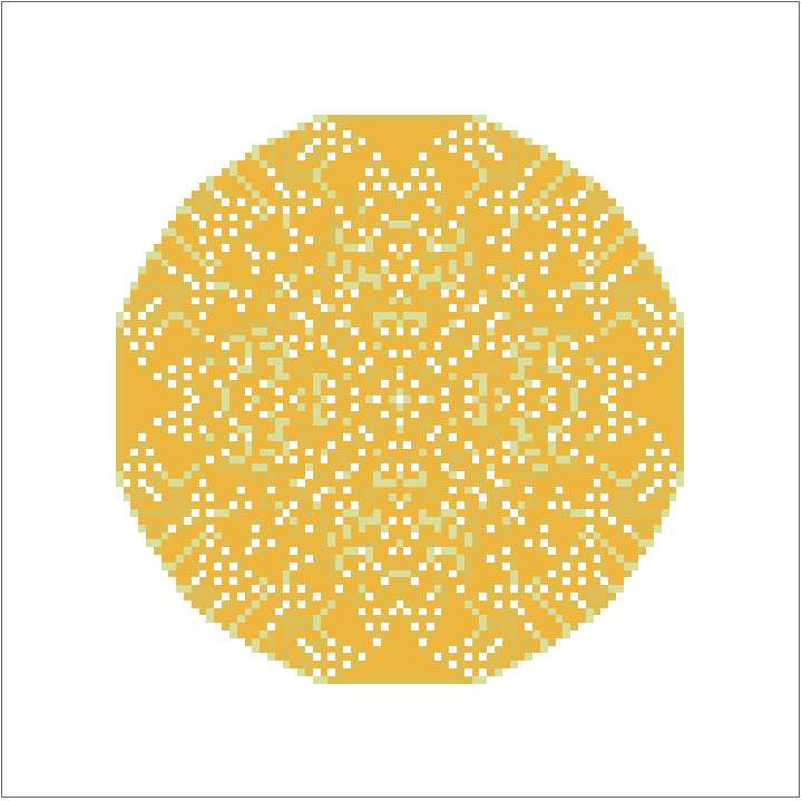
In my simulation, I modeled the sandpile on a 101×101 square lattice and initialized every site to state 0 so the entire grid began from the same inactive baseline.
Initializing the sandpile grid and tracking variables.
In[]:=
sand=ConstantArray[0,{101,101}];toppleCounts=ConstantArray[0,Dimensions[sand]];toppleEvents={};
I then repeatedly added a grain to the center site and called the update routine so the sandpile could relax after each addition.
The loop ran for 10, 000 iterations, while the live monitor displayed the current lattice using the plotting function, allowing me to observe how the pattern evolved over time.
The loop ran for 10, 000 iterations, while the live monitor displayed the current lattice using the plotting function, allowing me to observe how the pattern evolved over time.
Here sand is piled repeatedly onto the center site and the resulting sandpile is displayed.
Monitor[Table[sand[[51,51]]+=1;SandpileUpdate[];,{iter,10000}],sand//SandpilePlot]sand//SandpilePlot
Out[]=
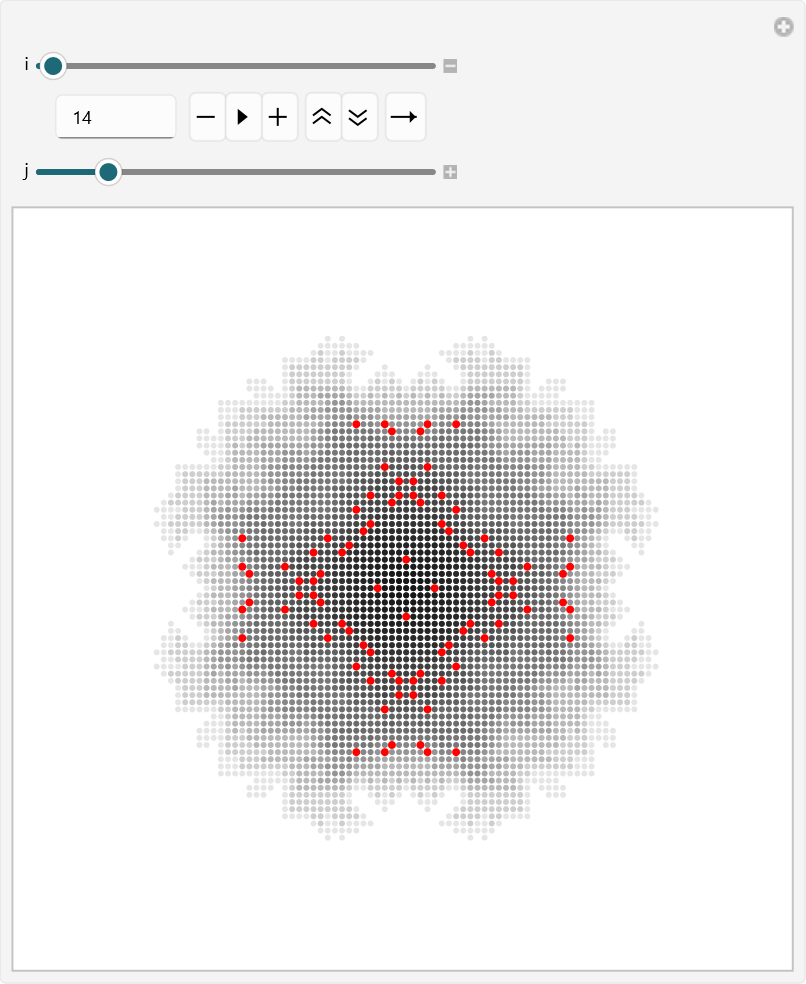
To examine the toppling behavior more closely, I used an interactive visualization that let me explore each cascade one at a time. The full set of points for a chosen toppling event was displayed faintly, while one selected point was highlighted in red so I could focus on a specific part of the event. This made it easier to see the internal structure of each cascade and observe how the affected sites were arranged within the lattice.
In my simulation, I used Manipulate to move through the sorted toppling events and inspect them interactively. The variable “i” let me choose which cascade to view, while “j” let me move through the points inside that cascade one by one. I also used “jSafe” to make sure the selected index stayed within bounds.
Interactive visualization of sorted toppling events with one highlighted point in each cascade.
Out[]=
To analyze the toppling data further, I used histograms to compare the sizes of individual toppling clusters and the total size of each cascade. This helped me study not only how many points were involved in each local cluster, but also how large the complete cascade became overall. By looking at both distributions, I could compare smaller, localized topplings with larger avalanche - like events across the sandpile.
I measured the lengths of the individual subclusters and plotted their frequency distribution.
I measured the lengths of the individual subclusters and plotted their frequency distribution.
Histograms of individual toppling cluster sizes and total cascade sizes.
cg21=toppleEvents//Map[Map@Length]//Flatten//Histogram[#,{1}]&
Out[]=
The first histogram shows the distribution of individual toppling - event lengths, and the main thing it reveals is that most toppling events are small but a few are exceptionally large. That means the model usually produced local cascades rather than very large spreading events, so toppling tended to happen in short bursts instead of running across the whole graph at once. In the graph, that would appear as repeated but limited pockets of instability rather than one dominant avalanche.
cg11=toppleEvents//Map[Map@Length]//Map[Total]//Histogram
Out[]=
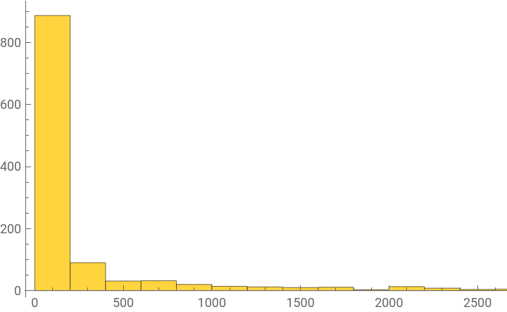
The cg11 histogram gives a slightly different view because it sums the lengths of the toppling events, so it shows the total amount of activity carried by each event. This makes the overall spread of activity easier to see, and it suggests that while many events were modest, a few were large enough to contribute much more heavily to the total dynamics. So instead of one uniform pattern, the process had a skewed structure where a smaller number of events did most of the work.
Taken together, the two results show that the sandpile process on this graph was not random noise. cg21 suggests that most cascades were short and local, while cg11 shows that the total activity still built up through a few stronger events.
That combination points to a system where the network supported repeated small - scale toppling, with occasional larger bursts that carried more weight in the overall behavior.
That combination points to a system where the network supported repeated small - scale toppling, with occasional larger bursts that carried more weight in the overall behavior.
Random Toppling
Random Toppling
Random toppling, also referred to as popcorn in this project, is a way of studying sandpile dynamics by adding grains to randomly selected sites instead of always using the center. This creates a less structured initiation pattern and allows the cascade behavior to be observed across the full lattice.
By comparing random toppling with center - based toppling, the model shows how the starting point of a disturbance can change the size, shape, and spread of the resulting cascade.
By comparing random toppling with center - based toppling, the model shows how the starting point of a disturbance can change the size, shape, and spread of the resulting cascade.
In my simulation, I began by creating a grid of zeros to represent the lattice, then stored the grid dimensions, initialized an array to count topplings at each site, and created an empty list to record the toppling events.
Initializing the sandpile grid and repeatedly adding grains to random sites while monitoring the evolving lattice.
After that, I repeatedly selected a random row and column, added one grain to that site, and called the update routine so the sandpile could relax after each addition.
I ran this process for 30, 000 iterations while using a live monitor to display the evolving lattice, which let me observe how the pattern changed over time as grains were added across different locations in the grid.
I ran this process for 30, 000 iterations while using a live monitor to display the evolving lattice, which let me observe how the pattern changed over time as grains were added across different locations in the grid.
To study the resulting cascades, I then sorted the toppling events by total size and used an interactive visualization to inspect them more closely. The faint gray points showed the full set of sites involved in each cascade, while the red point highlighted one selected site inside that event, making it easier to follow the internal structure of the toppling sequence.
Interactive visualization of sorted random toppling events with one highlighted point in each cascade.
Finally, I used histograms and a step plot to analyze the size distributions of the toppling events.
One histogram measured the sizes of individual toppling clusters.
The other measured the total size of each cascade, giving two complementary views of the same dynamics.
The step plot provided an additional way to see how the cascade sizes were distributed across the system.
Sandpile Dynamics on an n-Dimensional Hypercube
Sandpile Dynamics on an n-Dimensional Hypercube
Here the graph is set to HypercubeGraph[6], which means the sandpile is now being studied on a six - dimensional hypercube.
After defining the graph, I ran the random toppling simulation for 500 iterations and stored the results in data. I then animated the full evolution of the system using the recorded frames, which makes the toppling process easier to follow visually over time.
Running the randomized sandpile simulation on a six - dimensional hypercube and animating the resulting cascade behavior.
Using histogram and bar - based plots to summarize toppling counts on the hypercube graph.
The histogram showed that most of the values fall within a narrow high range, which means the vertices were being updated at fairly similar levels throughout the run. Rather than spreading widely across the full scale, the data clusters tightly, suggesting a strong degree of regularity in the toppling behavior.
The bar chart showed the same information more directly by preserving the activity level at each vertex. Most bars are close in height, but there are still small differences that show some vertices became slightly more active than others. This means the process was not completely uniform, even though the overall distribution remained tightly grouped.
The sorted bar chart makes the pattern easier to interpret by arranging the values from smallest to largest. In this form, the data appears to rise gradually rather than jumping sharply, which confirms that the toppling counts are closely packed together. The plot suggests that there are no extreme outliers dominating the process, only a relatively smooth spread of similar values.
Taken together, these results showed me that the randomized sandpile on the hypercube produces a highly concentrated and fairly stable pattern of activity. This suggests that the hypercube geometry supports a more even spread of activity than a system with more localized structure.
Sandpile Dynamics on a Two-Dimensional Hexagonal Lattice (2D Hexagonal Grid)
Sandpile Dynamics on a Two-Dimensional Hexagonal Lattice (2D Hexagonal Grid)
This section applies the same randomized sandpile process to a two-dimensional hexagonal lattice.
Random Toppling
Random Toppling
On a hexagonal lattice, the neighborhood structure differs from that of a square grid, so the spreading pattern of random toppling is not identical even though the update rule remains the same. That difference is important because it shows that the same model can produce different cascade behavior depending on the geometry of the graph. In this way, the hexagonal lattice serves as another example of how the sandpile framework adapts to new structures without changing the core logic of the simulation.
Defining a graph - based sandpile function with default iteration and threshold settings.
Running the randomized sandpile model on a two - dimensional hexagonal grid and collecting visual and statistical output.
The animation generated showed the evolution of the sandpile across all 1000 iterations. Visually, the frames illustrated how the pile grew, how unstable vertices were triggered, and how the activity moved through the lattice over time.
Animating the full sandpile evolution on the hexagonal grid over 1000 iterations.
Visualizing the data.
The histogram of the toppling data shows how the values are distributed across the vertices. The bars are concentrated within a fairly limited range, which suggests that many vertices experienced similar levels of toppling activity during the simulation. This kind of distribution indicates that the system developed a structured but not perfectly uniform pattern of activity.
The bar chart gives a direct view of the toppling counts at each vertex. Compared with the histogram, it preserves the individual vertex values more explicitly, so it is better for identifying which sites were more active than others. In this output, the bars reach a similar overall scale, but some are noticeably taller, showing that certain vertices accumulated more toppling activity than the rest.
This result reflects the irregular nature of random sand addition. Even though every vertex had the same chance of being selected, the repeated updates created local differences in activity over time. The bar chart therefore shows how randomness and threshold - driven redistribution combine to produce a nonuniform spatial pattern.
This result reflects the irregular nature of random sand addition. Even though every vertex had the same chance of being selected, the repeated updates created local differences in activity over time. The bar chart therefore shows how randomness and threshold - driven redistribution combine to produce a nonuniform spatial pattern.
The sorted bar chart arranges the same toppling values from smallest to largest. The sorted output shows how much variation exists in the data, and it makes it easier to see whether the counts rise gradually or whether there are sharp jumps in activity. The sorted bars show that many vertices fall into a comparable range, while a smaller number of sites stand out with higher values. That pattern is consistent with a system in which most sites experience moderate activity but a few sites accumulate more frequent toppling.
Centre toppling
Centre toppling
Here the sandpile is driven by repeatedly adding grains to one fixed center vertex instead of choosing random sites on a 2D Hexagonal Grid.
For the hexagonal lattice, the graph was defined as a 13 x 13 hexagonal grid, and the center vertex was set manually to vertex 167.
It was set manually because the center of a hexagonal lattice is not always unique in a discrete grid, especially when the lattice has an even number of rows and columns. Choosing the central vertex directly ensured that the simulation began from the most symmetrical point in the graph, which made the spreading pattern easier to interpret and kept the results consistent across runs.
The simulation was then run for 1000 iterations, so all of the sand accumulation begins from the same point and spreads outward through the lattice over time. The animation shows how the pile develops from that center point. Because the same vertex is being loaded repeatedly, the growth is much more concentrated than in the random toppling case. This makes the cascade easier to follow visually, since the toppling activity clearly radiates outward from one location rather than appearing in scattered places across the grid.
Running center - driven sandpile toppling on a hexagonal lattice with a fixed central vertex.
The histogram shows the distribution of the toppling counts across the vertices. The values are spread across a fairly wide range, with a noticeable concentration in the middle and upper regions of the graph. This means that many vertices were activated repeatedly during the simulation, especially as the cascade expanded outward from the center. Compared with the random toppling case, the histogram is less tightly clustered. That wider spread shows that center toppling produces stronger differences in vertex activity, since some parts of the lattice receive much more of the redistribution than others. In other words, the repeated input at one point creates a more uneven but also more structured distribution of toppling activity.
The bar chart gives a more direct view of the activity at each vertex. Here, a few bars rise much higher than the others, which shows that certain vertices experienced far more topplings than the rest. This is exactly what we expect from center driving, because the repeated stress at one site creates a stronger cascade near that region before the activity spreads outward. The uneven bar heights make the spatial structure of the toppling process easier to see. Instead of a mostly balanced spread, the graph shows clear peaks in activity, which means the pile is not distributing sand evenly across the lattice. The result is a more localized but more intense pattern of redistribution than the random case.
The sorted bar chart arranges the same values from smallest to largest, which makes the overall spread of the data easier to interpret. In this plot, the values rise gradually at first and then increase more sharply toward the upper end. That shape shows that many vertices had relatively low activity, while a smaller number of vertices accumulated very large toppling counts. This sorted form is useful because it makes the imbalance in the system more obvious. Instead of seeing the vertices in their original graph order, the plot highlights the range and concentration of values.
The result confirms that the center - driven process produces a much broader distribution than the more uniform cases seen earlier.
Overall, the center toppling results show a strongly focused avalanche pattern. Since every grain is added to the same vertex, the system builds up stress in one place and then releases it outward in repeated bursts.
Sandpile Dynamics on Graph-Based Networks
Sandpile Dynamics on Graph-Based Networks
Moving on to sandpile dynamics on graphs, the same basic threshold rule can be applied to a range of different network structures. This makes it possible to see how the arrangement of vertices and edges affects the way cascades form, spread, and settle over time. By using several graph-based layouts, the model can show how the same local process leads to different global patterns depending on the structure underneath it.
Sandpile Dynamics on Grid Graphs
Sandpile Dynamics on Grid Graphs
Sandpile dynamics on grid graphs provide a straightforward setting for observing how local threshold rules create larger cascade behavior across a network. In this part of the project, I used a 10 x 10 grid graph with labeled vertices and ran the random toppling sandpile process for 500 iterations. Because the grid has a regular structure, it gives a clear visual and numerical baseline for seeing how activity spreads through the system.
The animation shows the sandpile evolving over time as grains are added to random vertices and unstable sites topple. Since the graph is laid out in a simple square pattern, the movement of activity is easy to follow and makes the cascade process more readable. This helps show how the same rule can produce changing behavior even on a very regular network.
Running the randomized sandpile process on a labeled 10 x 10 grid graph for 500 iterations.
Creating an animation
The bar chart shows the toppling counts for each vertex. Most of the bars stay within a similar range, but a few are much taller, which means that some vertices were involved in more toppling activity than others. This suggests that while the activity is fairly spread out, it is not perfectly uniform across the grid.
Using a bar chart to show how toppling activity is distributed across the grid vertices.
The sorted bar chart arranges the same values from smallest to largest, making the distribution easier to interpret. It shows that many vertices experienced similar levels of activity, while only a smaller number reached much higher counts. Overall, the results show that the grid graph produces a balanced but still irregular pattern of toppling, making it a useful reference case for comparing with the other graph structures in the essay.
Sorting the vertex toppling counts to make the distribution of activity easier to read.
Sandpile Dynamics on Neural Graphs
Sandpile Dynamics on Neural Graphs
Sandpile dynamics on neural graphs provides a way to study how local threshold rules behave on irregular network structures rather than on a regular lattice. In this section, I used a random graph with 100 vertices and 300 edges, which gives a more complex and less structured setting for the sandpile process. Since the graph is not arranged in a simple geometric pattern, the results help us see how toppling behaves on a network that is closer to a general graph - based system.
Random Toppling
Random Toppling
Running the randomized sandpile process on a 100 - vertex random graph for 500 iterations.
The animation shows the evolution of the sandpile over 500 iterations as grains are added to random vertices and redistributed through the network. Because the graph is irregular, the pattern of activity is less predictable than in the grid or hexagonal cases. This makes the animation especially useful for showing how toppling spreads through a network whose connectivity is uneven.
The histogram shows that the toppling counts are concentrated in a limited range, with most values appearing in the lower to middle part of the distribution. This suggests that many vertices experienced moderate activity, while only a smaller number accumulated much larger counts. The bar chart shows the same result more directly, with a few bars reaching much higher than the rest, indicating that some vertices were involved in toppling far more often than others.
The bar chart shows the toppling counts at each vertex more directly, making it easier to identify which vertices were involved in more activity. While most bars remain relatively low, a few rise much higher, showing that the random driving created uneven toppling across the graph.
The bar chart shows the toppling counts at each vertex more directly, making it easier to identify which vertices were involved in more activity. While most bars remain relatively low, a few rise much higher, showing that the random driving created uneven toppling across the graph.
The sorted bar chart makes the distribution easier to read by arranging the values from smallest to largest. This reveals a clear spread in the data, with many vertices clustered at lower activity levels and a smaller set extending toward the upper end. Overall, the neural graph results show a more uneven and irregular pattern of toppling than the regular lattice cases, which reflects the randomness of the underlying network structure.
The sorted bar chart makes the distribution easier to read by arranging the values from smallest to largest. This reveals a clear spread in the data, with many vertices clustered at lower activity levels and a smaller set extending toward the upper end. Overall, the neural graph results show a more uneven and irregular pattern of toppling than the regular lattice cases, which reflects the randomness of the underlying network structure.
Network Pruning and Structural Refinement
Network Pruning and Structural Refinement
Neural Pruning
Neural Pruning
In neuroscience, pruning refers to the process by which the brain removes weaker, unnecessary, or less efficient synaptic connections during development and learning. This process helps refine neural circuits so that they become more specialized and efficient over time. The brain initially produces a surplus of connections, and pruning helps shape that broad network into a more organized system that supports effective communication between neurons. Rather than being a purely destructive process, pruning is an important part of normal brain development because it strengthens the overall structure of the network by keeping the most useful pathways and removing the ones that contribute less to function.
Effects of Underpruning and Overpruning
Effects of Underpruning and Overpruning
Underpruning and overpruning represent two opposite problems in this process. Underpruning happens when too many weak or unnecessary connections remain in the network, which can leave the circuitry overly dense and less refined. This may make the system less efficient because it contains more connections than it needs, and those extra connections can interfere with clear, specialized signaling. Overpruning, on the other hand, occurs when too many connections are removed, which can weaken communication between brain regions and reduce the network' s ability to function properly. In both cases, the issue is not simply the number of connections, but whether the balance of retention and removal supports healthy neural organization.
This is why pruning is often discussed in relation to connectivity loss and neurodevelopmental differences. If pruning is too weak, the brain may retain excess connections that make the network less streamlined; if pruning is too strong, important pathways may be lost, which can disrupt communication across the brain. Researchers have studied abnormal pruning as one possible factor in conditions involving atypical brain development, including autism, but it is important to be careful here because autism is not caused by pruning alone. Instead, it is a complex condition influenced by many factors, and pruning is only one part of a much larger developmental picture. Still, the idea of underpruning or overpruning is useful because it helps explain how changes in connectivity can affect brain function and development.
Structural Pruning of Isolated Vertices
Structural Pruning of Isolated Vertices
Structural pruning of isolated vertices is the process of simplifying a graph by removing vertices that are disconnected or only weakly attached to the main network. In a graph - theoretic or neuroscience - inspired setting, this means keeping the structure that actually contributes to overall connectivity while discarding parts that do not meaningfully interact with the rest of the system. The result is a cleaner and more coherent network, where the remaining vertices are more representative of the graph' s main structure. This kind of pruning is useful because it reduces unnecessary clutter without changing the essential connected core of the network.
the graph is first generated as a random network with 100 vertices and 175 edges. Because random graphs can contain isolated or weakly connected pieces, the initial structure may include disconnected leaves or small components that do not belong to the main network. The first step is therefore to keep only the largest connected component, which gives a more coherent base graph for the later pruning process.
Generating a random graph.
After extracting the largest component, the graph is repeatedly refined using a fixed - point pruning procedure. This means the pruning rule is applied again and again until no further structural changes occur. The result is a cleaner network in which disconnected or unnecessary parts have been removed, leaving only the main connected structure. Visually, the graph becomes more compact and better organized after pruning, with fewer stray vertices and a stronger overall connectivity pattern.
Extracting the largest connected component of a random graph and repeatedly pruning it until the structure stabilizes.
This is not activity - dependent pruning, since no sandpile dynamics or toppling counts are involved here. Instead, it is a purely structural form of pruning, where the goal is to simplify the network by removing weak or disconnected elements. That makes this section distinct from the earlier sandpile - based examples, because the focus is now on the graph' s geometry and connectivity rather than on dynamic activity across the network.
Activity - Dependent Synaptic Pruning
Activity - Dependent Synaptic Pruning
Activity - dependent pruning is a process in which a network is simplified by removing vertices or connections based on how much they participate in the dynamics of the system. In the context of this project, the idea is to run the sandpile model first, measure the toppling activity at each vertex, and then remove the least active parts of the graph. This makes the pruning rule dependent on behavior rather than just structure, because the network is being refined according to the activity it actually produced during the simulation.
Vertices that rarely topple are treated as less important to the overall dynamics, while vertices that are more active are preserved because they contribute more to the behavior of the system.
This type of pruning is useful because it creates a closer link between the structure of the graph and the dynamics occurring on it. Instead of deleting nodes randomly or only because they are disconnected, the graph is reduced according to the roles its vertices played in the sandpile process. That means the pruned graph is not just smaller, but also more selective, since it keeps the regions that were most involved in the cascade behavior. In a broader sense, activity - dependent pruning can be thought of as a way of extracting the most dynamically relevant part of a network, which makes it especially useful for studying how structure and behavior interact in graph - based models.
In Grid Graphs
In Grid Graphs
In this part of the project, the grid graph is pruned according to vertex activity after the sandpile simulation has been run. A 15 x 15 grid is first used as the initial network, and the sandpile process is applied for 1000 iterations to generate toppling counts for each vertex. The least active vertices are then identified from the sorted checklist and removed from the graph, producing a pruned network that preserves the parts of the structure most involved in the dynamics. This approach is called activity - dependent pruning because the pruning decision is based on how much each vertex participated in the sandpile process. As a result, the graph becomes a more refined representation of the network, with low - activity vertices removed and the more dynamically important parts retained.
Creating the grid graph.
Running the sandpile simulation on the grid graph and generate data for the experiment.
Finding the least active vertices.
Pruning the graph.
After pruning, the graph becomes noticeably more sparse and less uniform than the original grid. Most of the removed vertices come from the less active parts of the network, which are typically found near the edges and in regions that received fewer topplings during the simulation. The remaining structure keeps the more active vertices, so the pruned graph looks more concentrated around the areas that participated most in the dynamics. Instead of a full regular grid, the result is a thinner and more irregular network with gaps where low - activity vertices were removed. This shows that the pruning process does not remove vertices randomly; it selectively removes the parts of the graph that were least involved in the sandpile activity, leaving behind the more significant structural core.
In Neural Graphs
In Neural Graphs
Moving on to pruning these neural graphs, the same activity - based method can be used to remove the least active vertices and reveal a more refined network structure.
In this part, I again generated a random graph with 100 vertices and 175 edges was first generated, and then its largest connected component was extracted so that the pruning process began from a coherent network rather than a fragmented one. After that, the popcorn sandpile process was run for 500 iterations to measure how much activity each vertex received during the simulation. The output of the activity measurement was then sorted so that the least active vertices could be identified. These were the vertices with the smallest toppling counts, meaning they contributed least to the sandpile dynamics. The first ten vertices in that sorted list were selected for removal, and the graph was pruned by deleting them. This produced a smaller graph that retained the most active parts of the network while removing the weaker ones.
Generating a connected random graph running the sandpile process and deleting the least active vertices to create a pruned neural graph.
The pruned graph looks more compact and slightly less cluttered than the original network. Because the removed vertices were chosen based on low activity, the pruning does not affect the graph uniformly; instead, it tends to remove parts of the network that were less involved in the dynamics. In the visual output, this means that some peripheral or weakly connected regions disappear, while the more active core of the graph remains intact. This result shows that activity - dependent pruning can simplify a neural graph without destroying its main structural backbone. The remaining network is still connected and recognizable, but it is cleaner and more focused than the original graph. In that sense, the pruning highlights the vertices that played the most important role in the sandpile activity and removes those that contributed least.
Cascade Behavior in Pruned Networks
Cascade Behavior in Pruned Networks
In Grid Graphs
In Grid Graphs
In the pruned grid graph, the sandpile simulation was run again for 500 iterations on prunedGraph1, and the animation shows that cascades still propagated through the network, but within a smaller and more selective structure. Because the least active vertices had already been removed, the activity was forced to move through the remaining lattice, which made the propagation appear more concentrated than in the original grid. This suggests that pruning did not eliminate cascade behavior, but it did restrict where the activity could spread.
Running the sandpile process again on the pruned grid graph and pruned neural graph to observe how cascades behave after low - activity vertices have been removed.
In Neural Graphs
In Neural Graphs
In the pruned neural graph, the same procedure was applied to prunedGraph2 for 500 iterations. The resulting animation shows a more irregular cascade pattern, which is expected because the graph itself is nonuniform and was already simplified by removing low - activity vertices. Even after pruning, the network still supported toppling, but the activity followed the stronger surviving pathways rather than the weaker removed parts.
Running the sandpile process again on the pruned grid graph and pruned neural graph to observe how cascades behave after low - activity vertices have been removed.
Distribution of Cascade Responses Under Random Perturbation in Un-Pruned Neural Graphs
Distribution of Cascade Responses Under Random Perturbation in Un-Pruned Neural Graphs
In this section, I examined how the sandpile model behaved on a non-pruned random graph before any vertices were removed. The network was generated as a 100-vertex random graph with 175 edges, and the popcorn process was then repeated 10 times, each time for 500 iterations. This gave a collection of independent cascade runs on the same underlying graph, which made it possible to compare how propagation behaved when the full network was still intact.
Generating a random graph and running the sandpile process 10 times to compare propagation behavior in the non - pruned network.
Several experiments are run on the same graph to get a sample of its sandpile dynamics.
Plotted below are multiple bar charts and sorted bar charts that compare the spread of cascade activity across repeated non - pruned experiments.
The animations show that the cascades vary from run to run, even though the same graph is being used each time. Some experiments appear more concentrated, while others spread more broadly across the network, which reflects the randomness of both the graph structure and the grain - addition process. Because no pruning has been applied, the activity can move through the entire graph, including the weaker or less active regions that would later be removed in the pruned case. This makes the non - pruned network a useful baseline for seeing how cascades behave when the structure is still complete.
The bar charts show the toppling counts for each experiment, and they make it clear that the distributions are not identical from run to run. Some graphs show a sharper concentration of activity, while others are more spread out, but they all follow the same general pattern of a few more active vertices and many moderately active ones.
The sorted bar charts make this even easier to read because they arrange the values from smallest to largest, revealing the overall spread more clearly.
Taken together, these plots show that the non - pruned network supports flexible and variable propagation, since cascades are not restricted to a reduced core and can spread through the graph in multiple different ways.
Distribution of Cascade Responses Under Random Perturbation in Pruned Neural Graphs
Distribution of Cascade Responses Under Random Perturbation in Pruned Neural Graphs
In this section, I examined how the sandpile model behaved on the pruned neural graph after the least active vertices had already been removed. The same reduced network was used for 10 repeated experiments, and each run was carried out for 500 iterations. This made it possible to compare how cascade responses changed under random perturbation when the graph had already been refined into a smaller structural core.
The animations show that cascades still occur in the pruned network, but they spread through a more limited set of pathways. Because the weaker vertices were removed earlier, the activity is concentrated more strongly in the remaining parts of the graph. As a result, the propagation looks more focused and less diffuse than in the non - pruned case, while still retaining the irregularity expected from a random graph. This makes the pruned network a useful setting for seeing how cascade behavior adapts once the graph has been simplified.
The bar charts show the toppling counts for each experiment, and they make it clear that the distributions remain uneven across runs. Some trials produce stronger concentrations of activity at certain vertices, while others are more moderate, but the values stay within a similar range because the same pruned structure is reused each time.
The sorted bar charts make this easier to read by arranging the values from smallest to largest, which highlights the overall spread and shows that the activity is clustered rather than widely scattered. Taken together, these plots show that the pruned neural graph still supports cascade propagation, but the responses are now shaped by a smaller and more selective network.
Compared with the non - pruned case, the cascades are less broadly distributed and more constrained by the surviving structural core. This shows that pruning does not eliminate propagation, but it does change the way activity moves through the graph.
Spatial Distribution of Toppling Activity
Spatial Distribution of Toppling Activity
In this section, I used a heat map to visualize how often each vertex in the graph toppled during the sandpile process.
The aim was to represent the activity distribution more clearly by assigning both size and color to the vertices, so that more active sites would stand out immediately from less active ones. This makes the graph easier to interpret because it shows not only how much activity occurred, but also where that activity was concentrated within the network.
The plot maps the toppling counts onto a color gradient, with vertices that toppled more frequently appearing in warmer tones and vertices with fewer topplings appearing in cooler tones.
Vertex size was also scaled according to the same data, which reinforces the visual distinction between highly active and less active parts of the graph.
As a result, the heat map provides a compact summary of the cascade behavior and makes it easier to identify regions of strong toppling activity.
Creating a heat map graph that visualizes how many times each vertex toppled by mapping toppling counts to vertex size and color.
Color Key:
i) Dark blue lowest toppling activity, showing vertices that were only rarely or weakly involved in the cascade.
ii) Cyan to green low - to - moderate activity, where vertices toppled occasionally but not often enough to dominate the dynamics.
iii) Yellow moderate to high activity, marking vertices that were toppled repeatedly during the simulation.
iv) Orange high activity, showing vertices that participated strongly in the cascade process.
v) Red r highest toppling activity, marking the most frequently toppled and most dynamically active vertices in the graph.
The heat map result showed that toppling activity was not distributed evenly across the graph. Instead, a smaller number of vertices appeared in warmer colors, indicating that they were toppled more frequently, while cooler - colored vertices represented regions with lower activity. This made it possible to identify the most active parts of the network at a glance and see how the cascade concentrated in specific areas rather than spreading uniformly across all vertices.
Application to the C. Elegans Connectome
Application to the C. Elegans Connectome
I applied the sandpile model to the C. elegans connectome and observed how the system behaved as grains were added across the network. This allowed me to study the model on a real biological graph and see how the toppling process emerged within the connectome itself.
Why C.Elegans Connectome ?
Why C.Elegans Connectome ?
I chose to apply the sandpile model to C. elegans because it gave me a biologically grounded system that was still small enough to analyse in a clear and controlled way. Unlike a completely abstract graph, the C. elegans connectome represents a real neural network, so using it allowed me to explore how local instability and cascading activity might behave in an actual biological context. I also chose it because its connectome is exceptionally well mapped compared with many other organisms, which made it suitable for graph - based modelling and reduced the uncertainty that comes with incomplete network data. Another reason was that its size made it practical for detailed simulation: it was complex enough to produce interesting toppling behaviour, but not so large that the dynamics became impossible to interpret. By first pruning the network to its largest connected component, I ensured that the analysis focused on the main connected structure of the connectome, so the sandpile model could propagate meaningfully across the graph. This made C. elegans an ideal choice for demonstrating how the model worked on a real - world biological network rather than just on a theoretical example.
Methodology
Methodology
I began by loading the C. elegans connectome and restricting it to its largest connected component so that the analysis was performed on the main connected structure of the network. I then defined the sandpile model, assigned each vertex an initial sand count of zero, and repeatedly added grains to randomly chosen vertices. When a vertex reached the critical threshold, it toppled and redistributed sand to its neighbours, allowing cascades to develop across the graph. I recorded the number of top.plings at each vertex and visualised the results using bar charts, histograms, and an animated graph so that the spread of activity could be tracked over time.
Pruning the C. Elegans Connectome
Pruning the C. Elegans Connectome
Loads the full C. elegans connectome graph.
Finds the largest connected component in the graph.
Prunes the graph to only the largest connected component.
Examines the neighbourhood around vertex 18.
Displays the graph in 3D
Stores the total number of vertices in the graph.
Gets a list of all vertices.
Creates an association assigning zero sand to every vertex.
Random Toppling the Pruned the C. Elegans Connectome
Random Toppling the Pruned the C. Elegans Connectome
Running random sandpile toppling on a C. Elegans Connectome.
The sandpile simulation on C. elegans showed a clear pattern of uneven activity across the network, rather than a uniform spread of toppling everywhere. What stood out most was that some vertices kept becoming active much more often than others, which suggests that the structure of the connectome had a strong influence on where sand accumulated and where cascades began. In other words, the model did not treat every node equally: certain parts of the graph consistently played a larger role in the redistribution process.
This was especially visible in the histogram and bar chart. The histogram showed that the toppling values were not spread evenly across the full range, but instead clustered in a way that suggested most vertices experienced relatively limited activity, while a smaller number became much more involved. The bar chart made this even easier to see because it preserved the values for each vertex individually. There was a clear imbalance between vertices that barely toppled and those that contributed repeatedly to the cascade, which is exactly the kind of behaviour you would expect when a network has an uneven internal structure. The sorted bar chart reinforced this by showing a gradual rise in values rather than a dramatic jump, meaning the activity was distributed across the graph in a controlled but still noticeably unequal way.
The animation added another layer to the results because it showed the process unfolding over time. Some regions of the graph seemed to light up more often, while others remained relatively quiet, which gave a visual sense of how the connectome channels activity through certain areas more than others. That made the model feel less abstract and more like a dynamic process moving through a real network.
Overall, the results suggested that the C. elegans connectome supports structured cascade behaviour. The network did not respond randomly or evenly; instead, its own connectivity pattern shaped the toppling activity and created clear differences between vertices. This is important because it shows that the sandpile model can reveal something about the organisation of the connectome itself, not just the behaviour of the simulation. The main takeaway is that local toppling rules, when applied to a biological network like C. elegans, produce a non-uniform and highly structured pattern of activity that reflects the shape of the graph.
Results and Analysis
Results and Analysis
The main result of the project was that the sandpile model produced a highly uneven pattern of activity, which suggested that the network structure was doing most of the work rather than the random addition of grains itself. Once the threshold mechanism started operating, the model did not just spread sand uniformly through the graph. Instead, some vertices kept absorbing and redistributing sand more often than others, which meant that the same local rule produced very different outcomes depending on where it was applied in the network. That difference matters, because it shows that the topology of the graph was shaping the dynamics instead of the dynamics being independent of the graph.
In the random graph, this showed up as a fairly unstable but still structured cascade pattern. Vertices that were better connected or happened to sit in more influential positions were more likely to take part in repeated toppling, while other vertices stayed relatively inactive. That meant the model was not just producing random noise; it was exposing which parts of the graph were more capable of sustaining activity once the system was pushed past the threshold. The histogram and bar chart backed this up by showing that the distribution of toppling activity was not flat. Most vertices stayed low, but a smaller number accumulated much larger counts, which is exactly the kind of skew you would expect when local instability starts interacting with network structure.
The heat map added another layer to this, because it turned the toppling counts into a spatial pattern. Instead of looking at a list of numbers, it showed where the model was concentrating its activity. The warmer regions were not spread randomly across the graph, which suggests that the same vertices were repeatedly involved in the cascade process. That is important because it means the model was identifying structural “hot spots” in the network, places where activity was more likely to build up and trigger further topplings.
The C. Elegans connectome was where the project became most interesting, because the same rules were then being tested on a real biological network rather than an artificial one. After pruning the graph to its largest connected component, the model was applied to the main connected structure of the connectome, and the resulting dynamics again showed that activity was not evenly distributed. Some vertices took part much more often than others, which suggests that the connectome has its own internal organisation that affects how instability spreads.
The animation strengthened this interpretation because it showed the process unfolding over time rather than freezing it into a final state. What became clear from the animation is that toppling was not a one-off event but part of a repeating cycle of buildup, collapse, and redistribution. That matters because it shows the system was not settling into simple equilibrium; it was repeatedly moving between stability and instability. In other words, the model was capturing a dynamic process that depended on both the local threshold rule and the structure of the network it was running on.
Taken together, the results showed that the sandpile model was useful for revealing how cascades behave differently depending on the graph. On the random graph, it showed how instability can develop in a network with no biological meaning but clear structural constraints. On C. elegans, it showed that the same process can be mapped onto a real connectome and still produce uneven, structured activity. The overall pattern was that the network was not just a passive surface for the model, it actively shaped where cascades formed, how they spread, and which vertices ended up carrying the most activity.
Conclusion & Future Directions
Conclusion & Future Directions
Overall, this project showed that the sandpile model is a useful way of studying how local thresholds can create larger cascade effects across different types of networks. By testing it first on a random graph and then on the C. elegans connectome, I was able to see how the same simple rules produced different patterns depending on the structure of the graph. The random graph helped establish the basic behaviour of the model, while the connectome showed that the same process could be applied to a real biological network and still reveal uneven, structured activity. This made it clear that the topology of the network plays a major role in shaping where instability forms and how it spreads.
In future, this project could be extended by applying the model to other biological or real-world networks and comparing how cascade behaviour changes across different structures. It would also be useful to test different thresholds, redistribution rules, or starting conditions to see how sensitive the model is to changes in its parameters. Another possible direction would be to analyse the connectome in more detail by comparing different subgraphs or by measuring how centrality and connectivity relate to toppling frequency. That would make the analysis even stronger and help show more clearly how network structure influences dynamical behaviour.
In future, this project could be extended by applying the model to other biological or real-world networks and comparing how cascade behaviour changes across different structures. It would also be useful to test different thresholds, redistribution rules, or starting conditions to see how sensitive the model is to changes in its parameters. Another possible direction would be to analyse the connectome in more detail by comparing different subgraphs or by measuring how centrality and connectivity relate to toppling frequency. That would make the analysis even stronger and help show more clearly how network structure influences dynamical behaviour.
References
References
◼
Wolfram demonstrations project. (n.d.). https://demonstrations.wolfram.com/SandpileModel/
◼
Sandpile model for self-organized criticality. (n.d.). Wolfram Cloud. https://www.wolframcloud.com/obj/8e3b2b0b-10a1-4fb6-b797-6ae2dc40c706
◼
Risk, P. of. (n.d.). Sandpile model. Physics of Risk. https://rf.mokslasplius.lt/sandpile-model/
◼
Sakai, J. (2020). Core Concept: How synaptic pruning shapes neural wiring during development and, possibly, in disease. Proceedings of the National Academy of Sciences of the United States of America, 117(28), 16096–16099. https://doi.org/10.1073/pnas.2010281117
◼
What is synaptic pruning and why does your brain do it? (n.d.). Cleveland Clinic. https://my.clevelandclinic.org/health/articles/synaptic-pruning
Acknowledgements
Acknowledgements
It is often said that work of this kind is never the product of one person alone.
This project was shaped by the support, guidance, and generosity of many minds, and I am deeply grateful to everyone who contributed to it in one way or another.
First and foremost, I would like to thank my mentor, Dugan Hammock, for his incredible support throughout this project. I would also like to thank my advocate, Shenghui for helping me navigate the Wolfram Language at the start of the project. I am equally thankful to my TA, Amrita, for creating such a warm and supportive environment and Rory, Megan, Eryn, and Cyrus, the directors of WRSP, for all of their hard work in fostering such an inspiring environment for research and learning. I would also like to extend my thanks to every other staff member and TA at WRSP for their support, patience, and encouragement throughout the project and all of my fellow students for their friendship, support and companionship throughout the process.
Finally, I would like to express my gratitude to Stephen Wolfram for the opportunity and inspiration behind this project.
CITE THIS NOTEBOOK
CITE THIS NOTEBOOK
Modelling neuronal cascades with sandpile dynamics on synaptic connectivity graphs
by Gaurika Gautam
Wolfram Community, STAFF PICKS, July 9, 2026
https://community.wolfram.com/groups/-/m/t/3752237
by Gaurika Gautam
Wolfram Community, STAFF PICKS, July 9, 2026
https://community.wolfram.com/groups/-/m/t/3752237