The Computational Assyriologist — a three-part series.
Stephen Wolfram observes that for every field of science X there eventually emerges a computational X. This series asks what a computational Assyriology looks like: can we read the roughly nineteen thousand cuneiform tablets that carry no published translation (and most likely never had one) – and then study them not one at a time, but as a single corpus? The train of thought runs in three movements – first build the instrument, then learn to ask questions with it, then turn it loose on the whole archive:
◼ Part I — Building the translator: fine-tune a small, laptop-runnable Akkadian–English model (QLoRA), and measure honestly how well it reads.
◼ Part II — A research instrument (you are here): turn the translator into a Wolfram-Language research instrument – an atlas, social networks, intertextuality, omen logic, the Ark, a 763-BC eclipse.
◼ Part III — Reading nineteen thousand dark tablets: let a frontier model loose on the ~19,700 untranslated tablets (most likely never translated) and mine the whole library at once for names, places, stories and discoveries.
Each part stands on its own; the earlier parts build the tools used later. All code, data and build scripts are in the project repository.
Stephen Wolfram observes that for every field of science X there eventually emerges a computational X. This series asks what a computational Assyriology looks like: can we read the roughly nineteen thousand cuneiform tablets that carry no published translation (and most likely never had one) – and then study them not one at a time, but as a single corpus? The train of thought runs in three movements – first build the instrument, then learn to ask questions with it, then turn it loose on the whole archive:
◼ Part I — Building the translator: fine-tune a small, laptop-runnable Akkadian–English model (QLoRA), and measure honestly how well it reads.
◼ Part II — A research instrument (you are here): turn the translator into a Wolfram-Language research instrument – an atlas, social networks, intertextuality, omen logic, the Ark, a 763-BC eclipse.
◼ Part III — Reading nineteen thousand dark tablets: let a frontier model loose on the ~19,700 untranslated tablets (most likely never translated) and mine the whole library at once for names, places, stories and discoveries.
Each part stands on its own; the earlier parts build the tools used later. All code, data and build scripts are in the project repository.
Run this notebook. Download the bundle assyriologist_part2.wl attached to this post into the same folder as this notebook, then evaluate the cell below once. It loads every function and dataset used here, so each command cell underneath runs and reproduces its figure.
SetDirectory[NotebookDirectory[]];Get["assyriologist_part2.wl"]
10. The corpus in space and time — a cuneiform atlas
10. The corpus in space and time — a cuneiform atlas
Translation is only the start; the larger payoff is asking where and when the written record actually clusters. We harvested per-text metadata (provenience, period, genre) for 7,572 texts from eight ORACC projects, geocoded the find-sites, and mapped every text whose origin is known — 5,862 texts at 48 sites. This is built entirely in Wolfram Language (GeoGraphics over real archaeological coordinates) and is the substrate for everything spatial and temporal that follows. The map is one GeoGraphics call (full: community/build_atlas.wls):
GeoGraphics[bubble /@ sites, (* bubble ∝ text count, colour = region *)
GeoRange -> {{29.5, 37.8}, {38.5, 49.5}}, GeoBackground -> GeoStyling["ReliefMap"]]
GeoRange -> {{29.5, 37.8}, {38.5, 49.5}}, GeoBackground -> GeoStyling["ReliefMap"]]
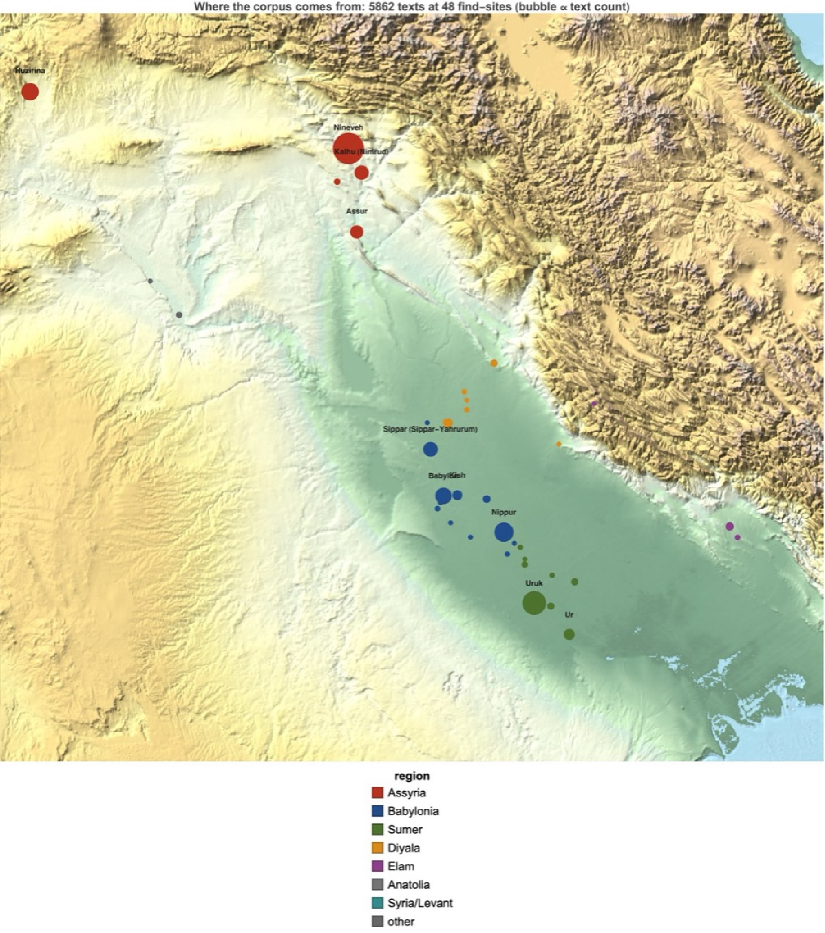
Figure 1. The corpus on the land. Each bubble is a find-site, sized by how many texts come from it and coloured by historical region. The picture is dominated by Nineveh (Ashurbanipal's library, the single richest source) and the Assyrian heartland (Assur, Kalhu), then Babylonia (Babylon, Sippar, Nippur) and the southern Sumerian cities (Uruk, Ur), with outliers in Elam (Susa) and Anatolia (Hattusa). This is as much a map of where archaeology and scholarship concentrated as of antiquity itself — a bias worth seeing explicitly before drawing historical conclusions.
How the map was built – and how complete it is. The atlas is a three-step chain, each reproducible. (1) harvest ORACC per-text metadata (study/harvest_meta.py corpus_meta.jsonl, 7572 texts, each with a provenience string like “Kuyunjik (Nineveh)”). (2) geocode those strings against a hand-checked gazetteer of tell coordinates (study/provenience_geocode.json, 91 sites from Pleiades / AWMC / excavation reports – the mound, not a nearby modern town). (3) plot in GeoGraphics. Honestly, geocoding places 81 of 90 distinct proveniences, covering 5864 of 7572 texts (77%) – the rest carry no usable find-spot and simply do not appear on the map:
geo = Import["study/provenience_geocode.json"]; (* provenience -> tell lat/lon *)
placed = Select[texts, KeyExistsQ[geo, #["provenience"]] &]; (* 5864/7572 have coordinates *)
GeoPosition[{geo[#["provenience"]]["lat"], geo[#["provenience"]]["lon"]}] & /@ placed
placed = Select[texts, KeyExistsQ[geo, #["provenience"]] &]; (* 5864/7572 have coordinates *)
GeoPosition[{geo[#["provenience"]]["lat"], geo[#["provenience"]]["lon"]}] & /@ placed
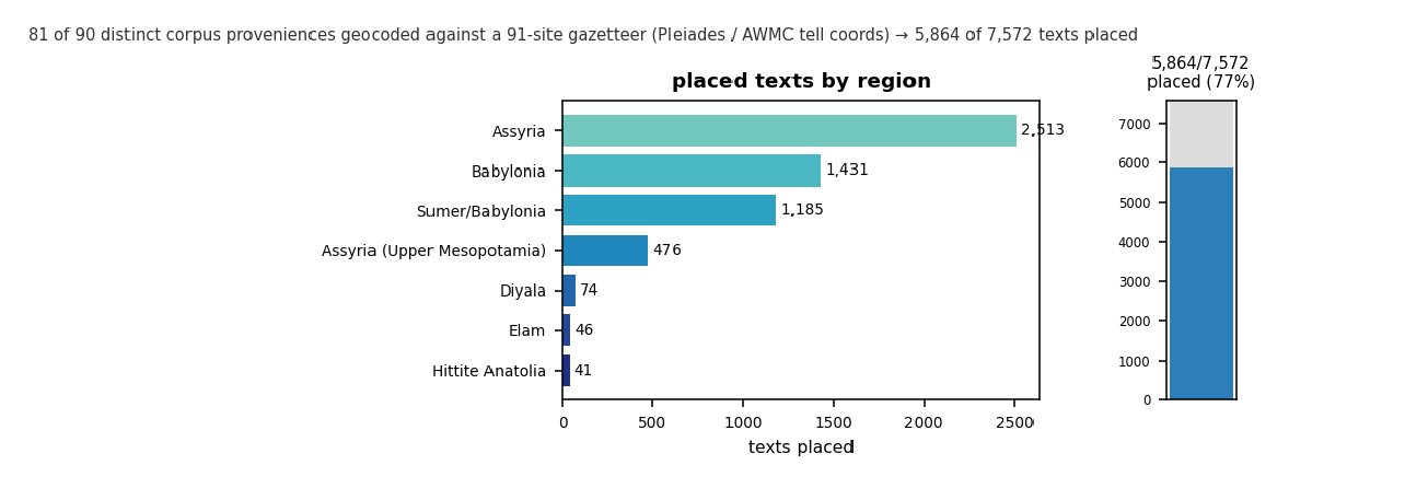
Figure 1b. Atlas coverage, honestly. The 5864 geocoded texts by region (Assyria leads, then Babylonia and Sumer), and the coverage bar: 77% of the corpus carries usable coordinates; the unprovenanced remainder is left off the map rather than guessed. Coordinates are the archaeological tells, from standard gazetteers.
Wolfram tool: a metadata join + GeoPosition / GeoGraphics over a hand-checked gazetteer – the reproducible spine under every spatial result in Parts II–III. Pipeline: study/analysis/atlas_pipeline.py.
The companion temporal view is one BarChart of text counts by period, ordered oldest-first – also from community/build_atlas.wls:
counts = textCountsByPeriod[atlas]; (* {Ur III, Old Babylonian, ..., Seleucid} *)
BarChart[Values[counts], ChartLabels -> Keys[counts], (* the Figure 2 period histogram *)
BarOrigin -> Bottom, ChartStyle -> byRegion]
BarChart[Values[counts], ChartLabels -> Keys[counts], (* the Figure 2 period histogram *)
BarOrigin -> Bottom, ChartStyle -> byRegion]
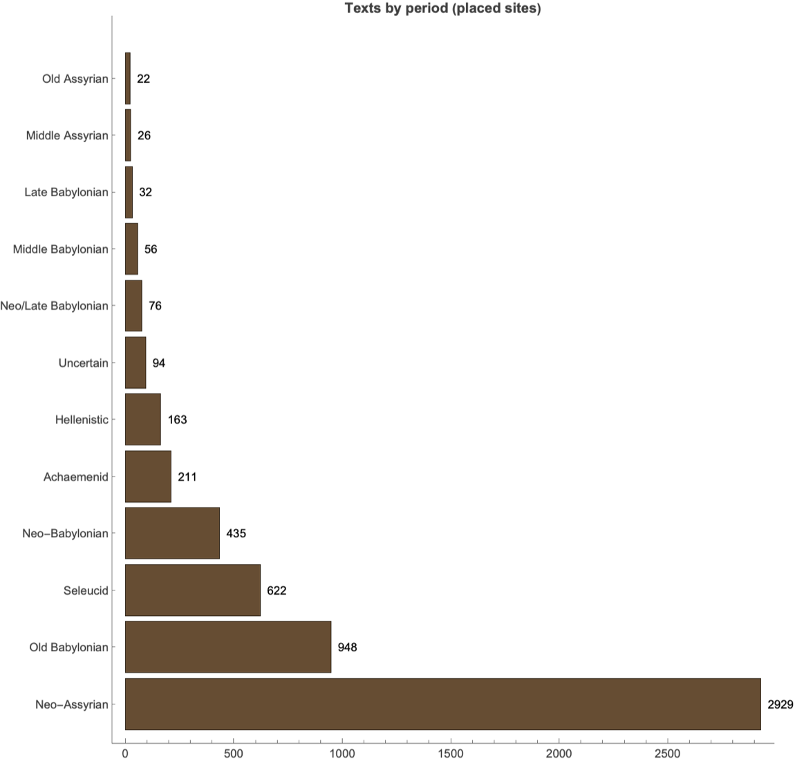
Figure 2. The corpus in time. Texts by period: a heavy Neo-Assyrian peak (the great 1st-millennium libraries), then Old Babylonian, Seleucid (late Uruk scholarship), and Neo-Babylonian. The corpus is a sampling of two great bursts — early-2nd-millennium Babylonia and 1st-millennium Assyria/Babylonia — not a uniform draw across three millennia.
Why this matters for the models. With every text now carrying a place and a period, we can move from description to process: animate text production across the map over time; test whether a linguistic or scribal feature is geographically clustered (spatial autocorrelation) or diffuses outward in a wave; and ultimately fit a reaction–diffusion model (NDSolve) for how an innovation spread along the Tigris–Euphrates. The atlas is the coordinate system for that work.
11. New investigations the pipeline enables
11. New investigations the pipeline enables
With translation, a metadata-rich corpus, and Wolfram in one place, the project becomes a research instrument, not just a translator. The point of this chapter is that one instrument – translate, geolocate, then compute in Wolfram – answers four different kinds of question about the same tablets, and we take them in turn:
• Textual – how stories relate and what is new: the three floods (§11.1), the cast of Gilgamesh as a network (§11.2), whether the flood was copied in a chain or a branching tree (§11.3), and fragments no one had translated (§11.4);
• Logical – testing the internal rules of a genre: omen polarity, with an exact statistical test (§11.5);
• Physical – reconstructing objects and games from their texts: the geometry of the round Ark (§11.6) and Finkel's Royal Game of Ur as a running program (§11.7);
• Chronological – pinning the calendar to the sky: the Bur-Sagale eclipse (§11.8).
Each is a real result built from real texts and the data on disk.
• Logical – testing the internal rules of a genre: omen polarity, with an exact statistical test (§11.5);
• Physical – reconstructing objects and games from their texts: the geometry of the round Ark (§11.6) and Finkel's Royal Game of Ur as a running program (§11.7);
• Chronological – pinning the calendar to the sky: the Bur-Sagale eclipse (§11.8).
Each is a real result built from real texts and the data on disk.
11.0 One instrument, many questions
11.0 One instrument, many questions
Before the four investigations, the claim itself deserves a demonstration. “One instrument” means a single parameterised function you can re-point at any slice of the corpus and get the same battery of views back. Define corpusSlice[genre, period] to return, for whatever slice you ask for, its find-sites, its timeline, and its characteristic words – then the rest of §11 is just this instrument pointed in different directions:
corpusSlice[genre_] := Module[{rows = corpusFilter[genre]},
Column[{
BarChart[siteCounts[rows]], (* WHERE: the find-sites *)
BarChart[periodCounts[rows]], (* WHEN: by period *)
BarChart[DeleteStopwords @ wordCounts[rows]] (* WHAT: content words *)
}]];
corpusSlice["Omen / divination"] (* one call all three views *)
Column[{
BarChart[siteCounts[rows]], (* WHERE: the find-sites *)
BarChart[periodCounts[rows]], (* WHEN: by period *)
BarChart[DeleteStopwords @ wordCounts[rows]] (* WHAT: content words *)
}]];
corpusSlice["Omen / divination"] (* one call all three views *)
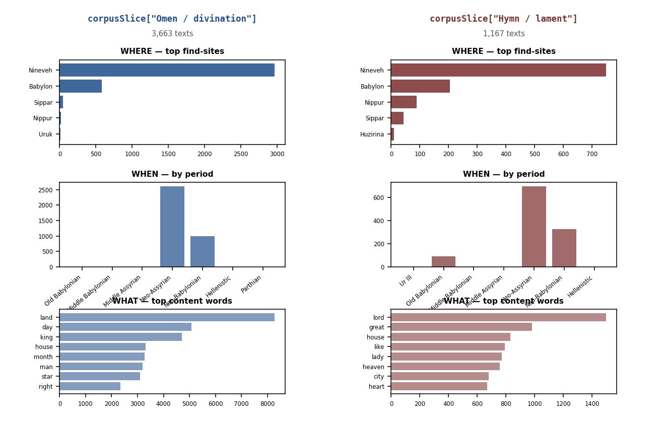
Figure 2b. The instrument, pointed two ways. The same corpusSlice function applied to two genres, returning all three views each – WHERE (sites), WHEN (period), WHAT (words). Omens resolve to the great libraries (Nineveh, Babylon, Sippar), a first-millennium peak, and the apodosis vocabulary (land, king, day); hymns & laments to Babylon and Nippur, an older spread, and a devotional vocabulary (lord, great, house). Same code, different input – the whole point of an instrument.
Wolfram tool: a parameterised slice the same three charts (site / period / word counts) for any genre, one function. The four sections that follow (§11.1–11.8) apply this same translategeolocatecompute pipeline to textual, logical, physical and chronological questions. Demo: study/analysis/corpus_slice.py.
11.1 Three floods: the Mesopotamian deluge and Genesis
11.1 Three floods: the Mesopotamian deluge and Genesis
The flood is the most famous cuneiform–biblical link. Using the actual texts – Gilgamesh XI and Atrahasis III (Akkadian), the Sumerian flood, the Old Babylonian Ark Tablet (Finkel 2014), and Genesis 6–9 – we align them motif by motif. The tightest parallel is the post-flood sacrifice and the god “smelling the sweet savour” (Gilg. XI 161–163 ≈ Gen 8:21); a concrete lexical link is bitumen kupru ≈ Hebrew kopher. The sharpest divergence is the ark's shape: one story, three incompatible geometries – a round coracle (Ark Tablet), a cube (Gilgamesh XI), and an elongated 6:1 box (Genesis) – direct evidence of distinct scribal traditions retelling the same plot.
A little history. This comparison is where Assyriology first met the public. In 1872 the self-taught British Museum scholar George Smith was reading a broken Kuyunjik tablet when he found a hero sending out a dove, then a swallow, then a raven from a grounded ship – a flood account older than Genesis. He reportedly leapt up and began undressing in his excitement. The sensation that followed (and the funded expedition that recovered the missing piece) launched cuneiform studies as a popular science. We can now line the texts up side by side and read them together: Gilgamesh XI is pulled live from the eBL (electronic Babylonian Library) API, and each motif becomes one colour-coded card (full data: study/flood_comparison.json):
gilgXI = URLExecute[ (* Gilgamesh XI, live from eBL *)
"https://www.ebl.lmu.de/api/fragments/K.3375/lines", "RawJSON"];
flood = Import["study/flood_comparison.json", "RawJSON"]; (* 5 sources x 10 motifs *)
floodCard /@ flood["motifs"] (* one Framed, colour-coded card per shared motif *)
(* tightest motif: post-flood sacrifice, the god "smells the sweet savour"
(Gilg. XI 161-163 ~ Gen 8:21); lexical link kupru ~ Hebrew kopher, "pitch" *)
"https://www.ebl.lmu.de/api/fragments/K.3375/lines", "RawJSON"];
flood = Import["study/flood_comparison.json", "RawJSON"]; (* 5 sources x 10 motifs *)
floodCard /@ flood["motifs"] (* one Framed, colour-coded card per shared motif *)
(* tightest motif: post-flood sacrifice, the god "smells the sweet savour"
(Gilg. XI 161-163 ~ Gen 8:21); lexical link kupru ~ Hebrew kopher, "pitch" *)
Figure 3. The flood narratives aligned motif by motif, on the actual texts (short quotes + citations, colour-coded by source / ark-geometry). Gilgamesh XI was pulled live from the eBL API; the Ark Tablet from Finkel, The Ark Before Noah (2014). Data: study/flood_comparison.json.
11.2 The cast of the Epic of Gilgamesh, as a network
11.2 The cast of the Epic of Gilgamesh, as a network
A trick borrowed from the study of novels and social media: treat a story's characters as nodes and their interactions as edges, then let the graph reveal the narrative's shape. We hand-curated the cast of the Standard Babylonian epic from A. R. George's edition – 25 characters and 40 ties (who fights, loves, parents, advises or kills whom, with the tablets each tie appears on) – and loaded it as a single Wolfram Graph. Two classical centrality measures then quantify what a reader feels: degree (how many others a character touches) and betweenness (how often a character lies on the shortest path between two others – a measure of “bridging” importance).
The numbers confirm the architecture. Gilgamesh and Enkidu dominate both measures (degree 16 and 10; betweenness 179 and 97) – the heroic first half, built on their friendship, is the structural core. The revealing third name is Utnapishtim: far behind on degree, but the highest-betweenness figure of the second half (betweenness 39, rank 3 overall). He is the narrow gateway through which Gilgamesh's quest for immortality reaches the flood survivor – so the graph literally exposes the epic's two-part design: a dense adventure cluster, then a thin bridge into the meditation on death. Data: study/gilgamesh_network.json; render: study/gilgamesh_network.wl:
g = Graph[edges, VertexSize -> degreeScaled, VertexStyle -> byClass];
bc = AssociationThread[VertexList[g], BetweennessCentrality[g]];
TakeLargest[bc, 3]
(* => <|Gilgamesh -> 179.4, Enkidu -> 97.0, Utnapishtim -> 39.3|>
Gilgamesh & Enkidu are the core; Utnapishtim is the bridge into the flood frame *)
bc = AssociationThread[VertexList[g], BetweennessCentrality[g]];
TakeLargest[bc, 3]
(* => <|Gilgamesh -> 179.4, Enkidu -> 97.0, Utnapishtim -> 39.3|>
Gilgamesh & Enkidu are the core; Utnapishtim is the bridge into the flood frame *)
Figure 4. Gilgamesh character network (25 nodes, 40 edges); node size = degree, colour = mortal / divine / monster / other. Data: study/gilgamesh_network.json.
The same method on real people: the king's correspondence. A network of a story's cast is one thing; the same instrument turned on real history is another. Beyond the eBL literary corpus we harvested the State Archives of Assyria – about 5036 letters to the Neo-Assyrian kings from their officials and scholars (free ORACC data, CC0). Each letter's catalogue records its sender and the reign it is dated to – and since these are letters to the king, that reigning king is in practice the recipient – so the archive is a social network: link every correspondent to the king(s) under whom they wrote. Out of 832 named senders the most prolific are exactly the famous inner circle – the chief scribe Issar-šumu-ereš, the exorcist Adad-šumu-uṣur, the astrologers Akkullanu and Balasî, and the king's agent in Babylon, Mar-Issar:
Figure 4b. Letters to the throne. The 48 best-attested correspondents (≥ 8 letters) of the Neo-Assyrian kings, each linked to the reign(s) they wrote under; node size ∝ surviving letters, colour = the king served, a dark ring marks the scholars whose careers bridged two reigns (Issar-šumu-ereš and Adad-šumu-uṣur advised both Esarhaddon and Ashurbanipal). The clusters are the courts of Sargon II and Esarhaddon – the two best-preserved archives. Metadata is the scholars’ (ORACC), not machine translation – exact for the attributed letters (see the honest-scope note below).
Honest scope. This is the shape of the preserved, attributed archive, not the whole Neo-Assyrian court. Only the 832 letters whose sender the editors could name enter the graph (many are anonymous or broken), and an edge is drawn only when the recipient king is unambiguous – letters dated “Esarhaddon or Ashurbanipal” are left out. So the network is a lower bound on the real correspondence, weighted toward the best-excavated reigns (Sargon II, Esarhaddon). What it shows is exact – these people did write these letters – but it is a floor, not a census. A fuller study would add the recipients-other-than-the-king and the people each letter names (a prosopography), which the catalogue also supports.
Wolfram tool: a two-mode Graph with an edge-weighted spring-electrical layout – the same network machinery as the Gilgamesh cast (§11.2), now over a real archive of 5036 letters. Digest (run on the harvest host): study/analysis/saa_network.py; figure in community/analysis.wl.
11.3 How the flood story travelled: linear chain or branching tree?
11.3 How the flood story travelled: linear chain or branching tree?
Scholars who edit ancient texts build a stemma – a family tree showing which copies descend from which – by grouping manuscripts that share distinctive readings. We can approximate that idea computationally: if we measure how similar each pair of flood stories is, the maximum spanning tree of those similarities is the simplest “family tree” linking them all. The question it answers is a real one in biblical and Mesopotamian scholarship: did the flood story descend in a straight line (Atrahasis Gilgamesh XI Genesis), or branch into related lineages?
We score pairwise similarity between the five sources – motif-overlap plus quote-level semantic similarity – and let FindSpanningTree build the tree. The answer is suggestive of branching, not a single chain: Atrahasis comes out as the hub (it ties directly to the Sumerian flood, Gilgamesh XI, and the Old Babylonian Ark Tablet), with Genesis attaching through Gilgamesh XI. That is consistent with Finkel's Ark-Tablet argument – the Ark Tablet as a distinct Old Babylonian witness inside the Atrahasis tradition (round coracle, “two by two”), not a point on a chain. A caveat worth stating: this is five texts and a two-decimal similarity matrix with several near-ties – the tree is suggestive, not a proof; a ±5% wobble in the scores can reshuffle the weakest edges. The topology falls out of the spanning tree (full script: community/build_flood_intertext.wls):
sim = Outer[combinedSim, sources, sources]; (* 0.5 motif-Jaccard + 0.5 quote-cosine *)
FindSpanningTree[Graph[srcPairs, EdgeWeight -> (1 - Flatten[sim])]]
(* MST: Atrahasis ties Sumerian, Gilgamesh XI, AND Ark Tablet (degree 3) -> BRANCHING *)
FindSpanningTree[Graph[srcPairs, EdgeWeight -> (1 - Flatten[sim])]]
(* MST: Atrahasis ties Sumerian, Gilgamesh XI, AND Ark Tablet (degree 3) -> BRANCHING *)
Figure 5. Left: combined-similarity heatmap (the Ark Tablet is the outlier; the Gilgamesh/Atrahasis/Sumerian/Genesis cluster sits at ~0.6). Right: the minimum-spanning tree – Atrahasis (purple) is the branching hub, Sumerian (green), Gilgamesh XI (blue), Ark Tablet (orange), Genesis (brown). Data: study/flood_intertextuality.md.
The method is worth unpacking, because it is the same three moves behind every “how related are these texts?” question in the series – turn each text into a vector, measure cosine similarity, keep the strongest links as a tree:
Figure 5b. How the family tree is built. Each text becomes a feature vector; similarity is the cosine of the angle between vectors (1 = identical content, 0 = nothing shared); the maximum spanning tree keeps the n−1 strongest links that connect everything without cycles. The worked pair shows the Ark Tablet sharing only 3 of the 10 motifs (cosine 0.55), which is why it hangs off to one side; the full score adds quote-level semantic cosine to separate the four complete tellings. A degree-3 hub (Atrahasis) means branching, not a single chain – exactly Finkel's reading.
Wolfram tool: cosine similarity + FindSpanningTree – the computational stand-in for a philologist's stemma. Figure stemmaMethodFigure in community/analysis.wl.
11.4 Reading texts with no published translation
11.4 Reading texts with no published translation
The real prize is the ~25,000 transliterated-but-untranslated fragments in the eBL Fragmentarium – our top novelty target (§11.9 maps the full landscape). As a proof of concept we harvested 76 fragments, biased toward literary, omen and myth material, that to our knowledge carried no published English, and ran every one through the local Gemma-4 fine-tune on the Mac mini (74 produced substantive drafts; 0 API errors). That is, to be honest, about 0.3% of the eBL pool – this is a demonstration of the workflow, not a cleared archive. But the workflow is the point: it turns a dark archive into a searchable first pass at zero marginal cost, and the same loop scales to the whole 25,000 unattended.
It already surfaces real content. The standout of the batch is SU-1951.19.A (Huzirina), which a frontier cross-read identifies with confidence as a manuscript of the Standard Babylonian Anzû epic – Ninurta's battle with the Anzû-bird – carrying a duplicate-note to the known witness STT 25. Others in the batch: a detailed bārû (diviner's) extispicy ritual to Šamaš and Adad (K.5408.A, catalogued only as “mythological, 20 lines”), an explanatory god-list centred on Nergal (BM.41255.C), and a vivid account of the destruction of Susa embedded in a geographical list (K.2035.A). Each is unvetted machine output – leads for an Assyriologist, not citable translations (the batch also contains clear errors, e.g. a menology where Gemma misread the DIš omen-marker as “Dishevelment”) – but these are exactly the leads a scholar wants. Each fragment is one call to the local model on the mini (free):
URLExecute[HTTPRequest["http://127.0.0.1:11435/api/generate", (* mini, Gemma-4 FT *)
<|Method -> "POST", "Body" -> ExportString[<|"model" -> "akkadian-gemma4",
"prompt" -> transliteration, "stream" -> False|>, "JSON"]|>], "RawJSON"]["response"]
<|Method -> "POST", "Body" -> ExportString[<|"model" -> "akkadian-gemma4",
"prompt" -> transliteration, "stream" -> False|>, "JSON"]|>], "RawJSON"]["response"]
(Fragmentarium drafts populate once the harvest+translation pass has run.)
Figure 6. Gemma-4 drafts of six previously-untranslated eBL fragments (tablet id • genre shown; drafts truncated). Unvetted machine output – the point is scale and discovery, not finality. Full batch of 76: study/fragmentarium_finds.md and study/fragmentarium_translated.json.
11.5 Omen logic: does “left” mean the enemy?
11.5 Omen logic: does “left” mean the enemy?
Divination was a science in ancient Mesopotamia – arguably its largest scholarly enterprise. Trained bārû priests read the future in the liver of a sacrificed sheep (extispicy), in the sky (the 70-tablet series Enūma Anu Enlil), in malformed births (Šumma izbu), in oil on water, in the behaviour of animals. Every omen has the same if–then shape: if a sign is seen (the protasis), then an outcome follows (the apodosis). Tens of thousands of these entries survive – a structured dataset two and a half millennia old.
A long-standing reading holds that spatial polarity encodes whose fortune is at stake: left (Akkadian šumēlu) for the enemy, right (imittu) for oneself – so a bad sign on the left is good news (it threatens them). Two questions, very different sample sizes. First, the big one – is the future mostly bad news? Over all 30,271 “if…” clauses, the apodoses that resolve either way are 85% unfavourable (6,132 bad to 1,063 good), worst of all for “the enemy” (451 bad : 2 good) and the army (398 : 19) – a real, large-n result (the subject×polarity test is in §12.12). Second, the narrow one – does left vs right predict whose fortune? Here the data nearly runs out: only ~30 omens carry both an unambiguous side-marker and a clear polarity. On those, both sides skew unfavourable (left 80%, right 93%) and a Fisher exact test gives p = 0.60 – which with n = 30 means underpowered, not refuted: we simply cannot tell whether the left = enemy rule holds. An honest “the data runs out here”, shown because it is as instructive as a result. Base Wolfram has no FisherExactTest, so we compute it directly from the HypergeometricDistribution (full script: community/build_omen_test.wls):
tbl = {{12, 3}, {14, 1}}; (* {left -> {unfav, fav}, right -> {unfav, fav}} *)
N[tbl[[All, 1]]/(Total /@ tbl)] (* unfavourable share: {0.80, 0.93} *)
(* Fisher's exact test, two-sided, straight from the hypergeometric: *)
{n, r1, c1} = {Total[tbl, 2], Total[tbl[[1]]], Total[tbl[[All, 1]]]};
d = HypergeometricDistribution[r1, c1, n]; pobs = PDF[d, tbl[[1, 1]]];
Total @ Select[PDF[d, #] & /@ Range[Max[0, r1 + c1 - n], Min[r1, c1]], # <= pobs &]
(* => 0.598 : not significant *)
N[tbl[[All, 1]]/(Total /@ tbl)] (* unfavourable share: {0.80, 0.93} *)
(* Fisher's exact test, two-sided, straight from the hypergeometric: *)
{n, r1, c1} = {Total[tbl, 2], Total[tbl[[1]]], Total[tbl[[All, 1]]]};
d = HypergeometricDistribution[r1, c1, n]; pobs = PDF[d, tbl[[1, 1]]];
Total @ Select[PDF[d, #] & /@ Range[Max[0, r1 + c1 - n], Min[r1, c1]], # <= pobs &]
(* => 0.598 : not significant *)
Figure 7. The ~30 omens carrying both an unambiguous side-marker and a clear polarity, by apodosis. Both the left (šumēlu) and right (imittu) columns are dominated by unfavourable outcomes (80% and 93%); the “left = enemy” rule predicts the opposite skew but the sample is far too small to tell (Fisher p = 0.60, n = 30 – underpowered, not refuted). The robust, large-n finding is the pervasive pessimism itself (85% of all 30,271 clauses skew bad). Data/figure: community/build_omen_test.wls, study/omens_analysis.md.
It is worth seeing the test itself, because the honesty is in the method. The whole claim rests on one 2×2 table – side against polarity – and a small-sample exact test, both shown here in full:
Figure 7b. The omen test, worked. The contingency table (left/right × unfavourable/favourable) with its margins, and the reasoning: because the smallest expected cell is far below 5, the χ² approximation would be unreliable, so we use Fisher's exact test – summing the exact hypergeometric probability of every table at least as extreme as observed. The result, p = 0.60 on n = 30, means the test is underpowered – we can neither confirm nor reject the famous left = enemy rule from the ~30 doubly-marked omens; the strong, real signal is the overall pessimism (§12.12).
Wolfram tool: a Fisher exact test built from HypergeometricDistribution (base Wolfram has no FisherExactTest) – the right test for small contingency tables, and transparent about why. Figure omenWorkedFigure in community/analysis.wl.
11.6 Does the Ark Tablet's round ark actually add up?
11.6 Does the Ark Tablet's round ark actually add up?
Finkel reads the Ark Tablet as a giant round coracle: floor area “one field” (1 iku), walls one nindan high, ~67–70 m across. Do the ancient units close? Converting (1 nindan = 12 cubits ≈ 6 m; 1 iku = 100 square nindan): the floor is 1 iku = 3,600 m^2, which is a circle of diameter 67.7 m – squarely inside Finkel's estimate. The tablet's numbers are internally consistent: area, diameter, wall height, and the stated bitumen (coating ~4,900 m^2 of hull) all cohere. It is a real, buildable – if enormous – guffa, not a literary flourish. The units close in three lines (full: study/ark_geometry.md):
nindan = 12 * Quantity[0.5, "Meters"]; (* 1 nindan = 12 cubits = 6 m *)
area = 100 * nindan^2; (* 1 iku = 100 square nindan = 3600 m^2 *)
2 * Sqrt[area/Pi] (* circle diameter = 67.7 m (Finkel: 67-70 m) *)
area = 100 * nindan^2; (* 1 iku = 100 square nindan = 3600 m^2 *)
2 * Sqrt[area/Pi] (* circle diameter = 67.7 m (Finkel: 67-70 m) *)
The cross-check goes further. The stated bitumen – 28,800 + 3,600 = 32,400 sutu – is about 194 m³ of pitch; spread over the 4,876 m² of floor-plus-wall it gives a waterproofing coat ~4 cm thick, exactly what you would actually apply. And a quiet surprise falls out of drawing all three arks to scale from their own numbers: the round coracle (3,600 m²) and the Gilgamesh cube (60 m a side also ~3,600 m²) have nearly the same floor area – it is Genesis, the long 6:1 box, that is the geometric outlier. Same flood, same scale, three very different hulls:
Figure 8. The three arks in plan, to scale from each text's measurements, with a football pitch (105 × 68 m) for reference. Ark Tablet (orange): round coracle, ⌀ 67.7 m. Gilgamesh XI (blue): a 60 m cube, 7 decks. Genesis (brown): a 150 × 25 m box. Each is enormous; the coracle and cube share a floor area, Genesis is the outlier. Figure + units: community/build_ark_geometry.wls, study/ark_geometry.md.
What might they have looked like? Here are 3D reconstructions of each text's hull (modelled in community/ark3d.nb). But a caveat the picture must not hide: the round coracle is Irving Finkel's reading of one Old Babylonian tablet (the Ark Tablet, 2014) – a striking and much-publicised proposal, but not the established reconstruction. The ark of tradition – the biblical 300×50×30-cubit vessel, and the great majority of scholarly and popular reconstructions – is a long box; the round reading applies only to that single Mesopotamian witness and is debated. These are illustrations of three texts, not a settled picture of “the” ark:
Figure 8b. Live 3D reconstructions of the three flood hulls – drag to rotate them. The Ark Tablet's round coracle (a coiled-rope guffa), the Gilgamesh XI cube (60 m, 7 decks), and the long Genesis box (150×25×15 m), each to its own text's proportions. The round form is Finkel's reading of one tablet, not the mainstream historical reconstruction – which, like the biblical ark, is a box. Built as Graphics3D in Wolfram Language; shown to convey shape, not to settle the debate.
11.7 Finkel's Royal Game of Ur, implemented in Wolfram Language
11.7 Finkel's Royal Game of Ur, implemented in Wolfram Language
One of the most charming chapters of Mesopotamian scholarship is Irving Finkel's decipherment of the rules of the Royal Game of Ur – a race game whose inlaid shell-and-lapis boards Leonard Woolley excavated from the Royal Cemetery at Ur in the 1920s, and which is now reckoned the oldest playable board game in the world (c. 2600 BC, some 4,600 years old). For decades the boards were mute: twenty beautiful squares, but no surviving rules. Finkel found them hiding in plain sight – a Babylonian clay tablet (BM 33333b) written by the scribe Itti-Marduk-balatu around 177 BC, which actually records how the game is played. Here is that game, reconstructed in Wolfram Language so you can run it yourself.
The rules (Finkel's reconstruction). Each player races 7 pieces along a 14-square track – private entry and exit squares either side of eight shared “war” squares. You move by the count on four binary (tetrahedral) dice, a Binomial(4, 1/2) over 0–4. Land on an opponent's unprotected piece on the shared lane and it goes back to the start; the five rosette squares are safe and grant another throw; a piece bears off only on an exact throw. First to bear off all seven wins. (On a two-player board only the central rosette is ever contested – the others sit on private tracks.)
The whole game is a short Wolfram program (community/game_of_ur.wl), and the same file exposes a live, playable board – urInteractive[]. Throw the dice, then click a highlighted blue stone to move it; you play the computer's greedy strategy (capture, else reach a rosette, else advance) – pure Wolfram, no model, no network:
Get["community/game_of_ur.wl"];
urRoll[] := Total @ RandomInteger[1, 4] (* four binary dice -> Binomial(4, 1/2) *)
urWinRates[100000] (* Monte-Carlo the balance (figures wobble ~1% per run): *)
(* => <|"p1WinRate" -> ~0.51, "meanRolls" -> ~120, "medianRolls" -> ~120|> *)
urInteractive[] (* the LIVE board: throw, then click a blue stone to move *)
urRoll[] := Total @ RandomInteger[1, 4] (* four binary dice -> Binomial(4, 1/2) *)
urWinRates[100000] (* Monte-Carlo the balance (figures wobble ~1% per run): *)
(* => <|"p1WinRate" -> ~0.51, "meanRolls" -> ~120, "medianRolls" -> ~120|> *)
urInteractive[] (* the LIVE board: throw, then click a blue stone to move *)
Figure 9. The Royal Game of Ur, live and playable. Press Throw the dice, then click a highlighted blue stone to move it; the red stones are played by the computer using a simple built-in greedy strategy (pure Wolfram, no model, no network). The layout is the canonical five-rosette board – in Finkel's rules every rosette (shaded) is a safe square and grants an extra throw, though on a two-player board only the central rosette is ever contested (the other four sit on private tracks). It is a self-contained DynamicModule, so it plays inside the saved notebook with nothing else loaded. Across simulated games the first player wins ≈ 51% – a slight first-mover edge, the exact figure wobbling about a percent from run to run – over a mean of roughly 120 dice throws (both players combined). Finkel's reconstructed rules give a genuinely balanced race. Code: community/game_of_ur.wl.
Why this matters. A philological decipherment cannot be run – but a game can. Turning Finkel's reading into executable code is a sanity check: had the rules produced a degenerate or hopelessly lopsided game, that would have counted against them. Instead they yield a playable, near-balanced race with captures and comebacks – consistent with Finkel's reconstruction. (A runnable game shows the rules are coherent, not that they are the correct ancient ones – that remains a philological judgement.)
11.8 Dating the chronology anchor: the Bur-Sagale eclipse
11.8 Dating the chronology anchor: the Bur-Sagale eclipse
How do we know that anything happened in 763 BC – or in any particular BC year at all? The Assyrians did not number years; they named each one after a high official, the līmu (eponym), and kept running lists of these names in order – the Assyrian Eponym Canon. That gives a continuous relative chronology (this year, then the next, for centuries) but no absolute pin: it floats, unless one entry can be tied to a datable event in the sky. One can. Beside the eponym of Bur-Sagale, the canon records that “the sun was eclipsed.” A total solar eclipse is visible from a strip of the Earth only tens of kilometres wide and recurs over a given city only once in centuries – so identifying which eclipse this was fixes that eponym, and with it the entire surrounding list, to the absolute calendar. This single line is the load-bearing anchor of first-millennium Mesopotamian chronology.
With Wolfram's astronomy we can check it directly. Scanning solar eclipses of 763–761 BC, exactly one is total over Assyria: a total eclipse on 7 June 763 BC (proleptic Gregorian) = 15 June 763 BC (Julian), magnitude 1.06, whose totality centerline passes ~167 km from Nineveh – well within this era's large, uncertain ΔT (Earth-rotation) budget. The date and the over-Assyria totality both match. The anchor of the chronology is confirmed astronomically – the kind of cross-check only a computational-astronomy engine makes routine. The whole result is a handful of built-in calls (full script: community/build_eclipse_map.wls):
seed = DateObject[{-763, 6, 1}, TimeZone -> 0]; (* scan from June 763 BC *)
SolarEclipse[seed, "MaximumEclipseDate"] (* -> 7 Jun 763 BC (= 15 Jun Julian) *)
SolarEclipse[seed, "Type"] (* -> Total *)
SolarEclipse[seed, "Magnitude"] (* -> 1.06 *)
GeoDistance[GeoPosition[{36.36, 43.15}], (* Nineveh *)
SolarEclipse[seed, "TotalPhaseCenterLine"]] (* -> Quantity[167, "Kilometers"] *)
SolarEclipse[seed, "MaximumEclipseDate"] (* -> 7 Jun 763 BC (= 15 Jun Julian) *)
SolarEclipse[seed, "Type"] (* -> Total *)
SolarEclipse[seed, "Magnitude"] (* -> 1.06 *)
GeoDistance[GeoPosition[{36.36, 43.15}], (* Nineveh *)
SolarEclipse[seed, "TotalPhaseCenterLine"]] (* -> Quantity[167, "Kilometers"] *)
Figure 10. The total solar eclipse of 7 June 763 BC (= 15 June Julian): the totality band over Mesopotamia, crossing just over Nineveh (~167 km from the centerline). Grey dots = corpus find-sites. Data: study/eclipse_verification.md.
11.9 How much is still in the dark? A census of the untranslated record
11.9 How much is still in the dark? A census of the untranslated record
§11.4 dipped into the eBL Fragmentarium; this section steps back and measures the whole gap. How many cuneiform texts exist as scholarly transliterations but have never been put into English? We did not estimate – we downloaded the bulk files and counted translation status directly. For ORACC we parsed the trans field of all 57 project catalogues; for CDLI we grepped 135,254 transliterated texts for any #tr.en line (only ~4% had one); for BDTNS and eBL we parsed the published bulk exports. The result is sobering and motivating in equal measure:
The deduped, transliterated-but-untranslated pools total ~340,000 texts. The two largest are administrative – CDLI (~130k) and BDTNS (~76k Ur III), formulaic but priceless for economic and social history and highly learnable by MT. The ORACC edition corpora (~57k) are the cleanest input, already lemmatised. And the eBL Fragmentarium (~25k, only ~0.7% translated) holds the highest odds of genuinely new literary content – unplaced Gilgamesh lines, new omens, commentaries (the Anzû manuscript of §11.4 came from exactly here). Each is a concrete target the local translator can attack offline, at zero marginal cost. The census is one BarChart (full method: study/untranslated_pools.md; figure: community/build_pools_census.wls):
pools = {{"CDLI bulk ATF", 130}, {"BDTNS (Ur III)", 76}, {"ORACC editions", 57},
{"Archibab (OB)", 30}, {"NaBuCco (NB)", 26}, {"eBL Fragmentarium", 25}}; (* thousands, MEASURED *)
BarChart[Labeled[#[[2]], #[[1]], Left] & /@ ReverseSortBy[pools, Last], BarOrigin -> Left]
(* total deduped untranslated pool: ~340,000 transliterated texts with no English *)
{"Archibab (OB)", 30}, {"NaBuCco (NB)", 26}, {"eBL Fragmentarium", 25}}; (* thousands, MEASURED *)
BarChart[Labeled[#[[2]], #[[1]], Left] & /@ ReverseSortBy[pools, Last], BarOrigin -> Left]
(* total deduped untranslated pool: ~340,000 transliterated texts with no English *)
Figure 11. The dark archive, by pool (thousands of transliterated texts with no published English; counts measured from the bulk files, not estimated). Blue = the project's primary discovery targets. The administrative bulk (CDLI + BDTNS) is the volume; the eBL Fragmentarium is the best bet for new literary finds. Data: study/untranslated_pools.md.
11.10 Open questions this stack could actually move
11.10 Open questions this stack could actually move
None of the above is an end in itself. Bulk local translation, a geocoded metadata-rich corpus, and Wolfram in one place is really a research instrument pointed at live scholarly debates. We compiled a ranked, sourced list of open questions the stack could plausibly contribute to (study/open_questions.md); the most tractable are already half-built from the data on disk:
• Shared canon or local networks? Oppenheim's “stream of tradition” is often treated as a universal canon; Robson and others argue scholarship was locally inflected. Our corpus_meta.jsonl links 7,572 texts to composition, period and geocoded site – enough to build a bipartite site ↔ composition graph and run FindGraphCommunities to test “universal vs local” quantitatively.
• Which dates are astronomically over-determined? §11.8 re-derived the Bur-Sagale anchor; the same method extends to VAT 4956 (year 37 of Nebuchadnezzar II), whose ~13 lunar + 15 planetary positions make its year unique – a second independent chronology check.
• Authorship and editorial history of Standard Babylonian Gilgamesh – stylometry over the eBL line corpus (§9 already aligns our drafts to George's edition).
• Prosopography from the untranslated mass – names, places and transactions extracted from the ~100k Ur III administrative pool (§11.9) feed social-network and commodity-flow history.
• The pace and geometry of the Aramaic shift – a spatial-temporal “language-death clock” for when and where cuneiform yielded to alphabetic Aramaic.
• Which dates are astronomically over-determined? §11.8 re-derived the Bur-Sagale anchor; the same method extends to VAT 4956 (year 37 of Nebuchadnezzar II), whose ~13 lunar + 15 planetary positions make its year unique – a second independent chronology check.
• Authorship and editorial history of Standard Babylonian Gilgamesh – stylometry over the eBL line corpus (§9 already aligns our drafts to George's edition).
• Prosopography from the untranslated mass – names, places and transactions extracted from the ~100k Ur III administrative pool (§11.9) feed social-network and commodity-flow history.
• The pace and geometry of the Aramaic shift – a spatial-temporal “language-death clock” for when and where cuneiform yielded to alphabetic Aramaic.
A caveat frames all of these: the field's measured bottleneck is not headline BLEU but faithfulness – Gutherz et al. (2023) found human judges accepted only ~40–44% of an NMT system's outputs as proper translations even at BLEU ~37. So every MT-driven claim here is paired with model-disagreement flagging plus frontier verification on flagged lines, and nothing is published without expert review. These are leads and instruments, not verdicts.
— End of Part II — A research instrument —
— End of Part II — A research instrument —
In Part II the translator became an instrument. With a metadata-rich corpus in Wolfram Language we mapped where the tablets were found and when; compared the flood across Gilgamesh, Atrahasis, the Sumerian flood and Genesis; drew the cast of Gilgamesh and the king's correspondents as social networks; tested whether textual transmission was linear or branching; weighed omen logic with an exact statistical test; checked the geometry of the round Ark; rebuilt the Royal Game of Ur as a playable program; and pinned the Bur-Sagale eclipse to 7 June 763 BC to anchor the chronology. Every section foregrounds the Wolfram tool it uses.
Coming next – Part III — Reading nineteen thousand dark tablets. So far we have read tablets a handful at a time. In Part III we let the translator loose on the whole eBL Fragmentarium – ~19,700 fragments that carry no published translation (and, as far as we can tell, were probably never translated) – and read the entire library at once: what it is about, who appears in it, where and when, how the script drifts over time, the stories it hides, the cuneiform behind them, and the candidate joins and discoveries it surfaces. One honest shift of gears: where Parts I–II showcased the model you own, Part III's bulk drafting leans on a frontier model – claude-opus-4-8 for the ~2,000 most substantial fragments, claude-haiku for the broken remainder – because the local Gemma fine-tune comes back ~85% garbled on dense first-millennium scholarly tablets.
Coming next – Part III — Reading nineteen thousand dark tablets. So far we have read tablets a handful at a time. In Part III we let the translator loose on the whole eBL Fragmentarium – ~19,700 fragments that carry no published translation (and, as far as we can tell, were probably never translated) – and read the entire library at once: what it is about, who appears in it, where and when, how the script drifts over time, the stories it hides, the cuneiform behind them, and the candidate joins and discoveries it surfaces. One honest shift of gears: where Parts I–II showcased the model you own, Part III's bulk drafting leans on a frontier model – claude-opus-4-8 for the ~2,000 most substantial fragments, claude-haiku for the broken remainder – because the local Gemma fine-tune comes back ~85% garbled on dense first-millennium scholarly tablets.
Reproducible end to end – data build, QLoRA training, GGUF/Ollama export, benchmark, batch translator and this notebook (community/build_notebook.wls) are all in the repository. Text data: ORACC (CC BY-SA 3.0) and the electronic Babylonian Library / eBL (CC BY-NC-SA 4.0), reused with attribution for non-commercial research; the derived data and this notebook are shared under CC BY-NC-SA 4.0. Method: Akkademia; Gutherz et al. (2023). Machine translations are leads for specialists, not citable readings.
CITE THIS NOTEBOOK
CITE THIS NOTEBOOK
The computational assyriologist - Part II: cuneiform as a research instrument
by Marco Thiel
Wolfram Community, STAFF PICKS, June 17, 2026
https://community.wolfram.com/groups/-/m/t/3735072
by Marco Thiel
Wolfram Community, STAFF PICKS, June 17, 2026
https://community.wolfram.com/groups/-/m/t/3735072