Non-Newtonian Fluid Model Determination
Authors: Housam Binous and Ahmed Bellagi
Authors: Housam Binous and Ahmed Bellagi
Reference:
H . Binous, Introducing non-Newtonian fluid mechanics computations with Mathematica® in the undergraduate curriculum, Chemical Engineering Education, 41 (1), pp . 59 - 64, 2007.
H . Binous, Introducing non-Newtonian fluid mechanics computations with Mathematica® in the undergraduate curriculum, Chemical Engineering Education, 41 (1), pp . 59 - 64, 2007.
Non-Newtonian fluid model determination using experimental flow rate values measured under different applied pressure gradients in a horizontal pipe of radius a=0.01 m.
Reference: Problem 15 Chapter 11 Page 553 of textbook by J. O. Wilkes, Fluid Mechanics for Chemical Engineers, Prentice Hall, 1999.
Reference: Problem 15 Chapter 11 Page 553 of textbook by J. O. Wilkes, Fluid Mechanics for Chemical Engineers, Prentice Hall, 1999.
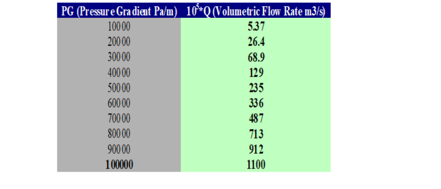
Determination of Bingham Fluid Parameters: =tau0 and =visc using experimental data.
τ
0
μ
0
Expression of the Volumetric Flow Rate for Bingham Fluids with =
Q=1-+
ΔPπ
4
a
8L
μ
0
4
τ
0
3
τ
R
1
3
4
τ
0
τ
R
τ
R
ΔPR
2L
In[]:=
QBingham[PressureGradient_]:=Pia^4/(2visc)(PressureGradient)(1/4.-β[PressureGradient]/3+β[PressureGradient]^4/12)
In[]:=
β[PressureGradient_]:=2tau0/(aPressureGradient)
In[]:=
EXPRESSION1=QBingham[PressureGradient]
Out[]=
4
a
2tau0
3aPressureGradient
4
4
tau0
3
4
a
4
PressureGradient
2visc
Experimental data
In[]:=
mydata={{10^4,5.3710^-5},{210^4,2.6410^-4},{310^4,6.8910^-4},{410^4,1.2910^-3},{510^4,2.3510^-3},{610^4,3.3610^-3},{710^4,4.8710^-3},{810^4,7.1310^-3},{910^4,9.1210^-3},{10^5,1.1110^-2}};
Calculation of the Sum of Squares
In[]:=
sumOfSquares[data_]:=Apply[Plus,Apply[Plus,Map[{(QBingham[#[[1]]]-#[[2]])^2}&,data]]]
In[]:=
myEvaluater[tau0_,visc_,data_]:=sumOfSquares[data]
Pipe Radius
In[]:=
a=0.01;
Wefind=77.55and=0.0326
τ
0
μ
0
In[]:=
paramBingham=FindMinimum[myEvaluater[tau0,visc,mydata],{tau0,0.1,90},{visc,.01,1000},MaxIterations300]
Out[]=
{9.88786×,{tau077.55,visc0.0326486}}
-6
10
Same calculation as above this time using the built-in command NonlinearModelFit yields the same values for Bingham Fluid Parameters: and
τ
0
μ
0
In[]:=
nlm1=NonlinearModelFit[mydata,EXPRESSION1,{tau0,visc},PressureGradient]
Out[]=
FittedModel
In[]:=
nlm1["ParameterTable"]
Out[]=
Estimate | Standard Error | t-Statistic | P-Value | |
tau0 | 77.5494 | 11.032 | 7.02947 | 0.000109379 |
visc | 0.0326483 | 0.0026468 | 12.335 | 1.7376× -6 10 |
In[]:=
nlm1["RSquared"]
Out[]=
0.967036
Determination of Power Law Fluid Parameters: n and k using experimental data.
In[]:=
a=.;
Expression of the Volumetric Flow Rate for Power Law Fluids
Q=nπ
3+
1
n
a
1
n
ΔP
2kL
1+3n
In[]:=
QPowerLaw[PressureGradient_]:=(PressureGradient/(2k))^(1/n)Pina^(3+1/n)/(1+3n)
In[]:=
EXPRESSION2=QPowerLaw[PressureGradient]
Out[]=
-1/n
2
3+
1
n
a
1
n
PressureGradient
k
1+3n
Calculation of the Sum of Squares
In[]:=
sumOfSquares[data_]:=Apply[Plus,Apply[Plus,Map[{(QPowerLaw[#[[1]]]-#[[2]])^2}&,data]]]
In[]:=
myEvaluater[n_,k_,data_]:=sumOfSquares[data]
Pipe Radius
In[]:=
a=0.01;
Wefindn=0.437andk=6.708
In[]:=
param1=FindMinimum[myEvaluater[n,k,mydata],{n,0.42,0.5},{k,6,10},MaxIterations100000]
Out[]=
{2.67047×,{n0.437422,k6.70852}}
-7
10
Same calculation as above this time using the built-in command NonlinearModelFit provides similar values for Power law Fluid Parameters: and
n
k
In[]:=
nlm2=Quiet@NonlinearModelFit[mydata,{EXPRESSION2,n>=0,k>=0},{n,k},PressureGradient]
Out[]=
FittedModel
In[]:=
Quiet@nlm2["ParameterTable"]
Out[]=
Estimate | Standard Error | t-Statistic | P-Value | |
n | 0.435014 | 0.0113486 | 38.3318 | 2.35641× -10 10 |
k | 6.85783 | 0.710385 | 9.65368 | 0.0000110363 |
In[]:=
nlm2["RSquared"]
Out[]=
0.999105
Plot of the volumetric flow data versus pressure gradient for both model
In[]:=
Show[ListPlot[mydata,PlotStyle{Thick,Darker@Green,PointSize[0.02]},Frame->True,AspectRatio->1,FrameLabel->{Style["pressure gradient (Pa/m)",14],Style["volumetric flow rate ( /s)",14]},GridLines->Automatic,ImageSize->400{1,1},FrameTrue],Plot[{nlm2[x],nlm1[x]},{x,10000,100000},PlotLegends->{Style["power law",14],Style["bingham",14]}]]
5
10
3
m
Out[]=
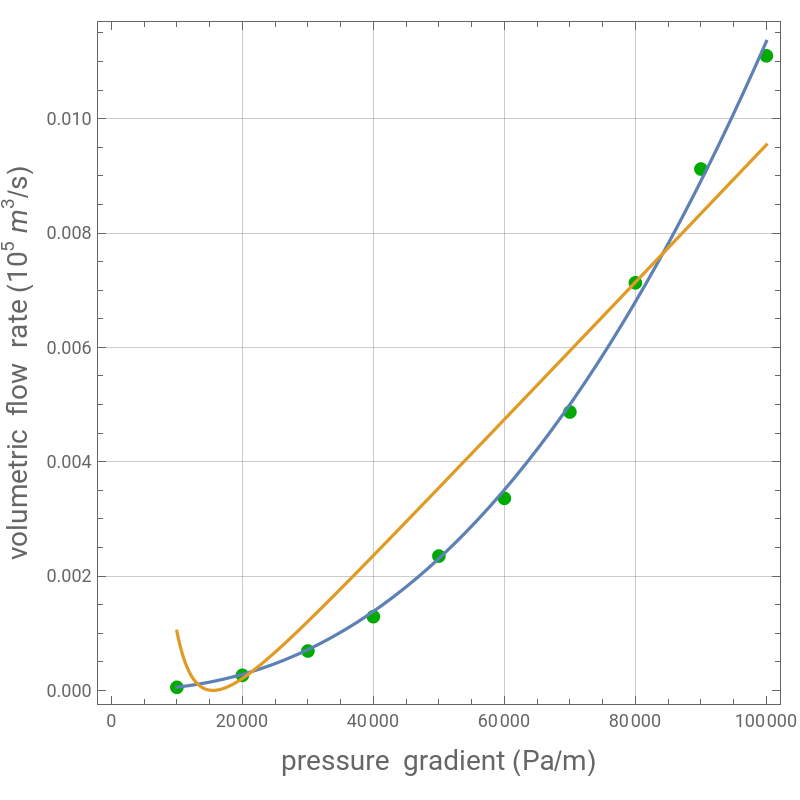


A visual check as well as the values found above (0.9670 and 0.9991) lead us to the conclusion that Power Law model fits better experimental data
2
R