Unsteady Diffusion Problem in Spherical Coordinates using the Orthogonal Collocation Method
Authors: Housam Binous and Ahmed Bellagi
Unsteady Diffusion Problem in Spherical Coordinates using the Orthogonal Collocation Method
Authors: Housam Binous and Ahmed Bellagi
Authors: Housam Binous and Ahmed Bellagi
Acknowledgement :We study the problem treated by W. F. Ramirez (Ref. 1). The governing equation, boundary conditions and initial condition are given by :=D with ,IC : ,BC1 : =0,BC2 : at ,References :[1] W. F. Ramirez, Computational Methods for Process Simulation, Second Edition, 1997, Butterworth Heinemann, Oxford.
∂c
∂t
1
2
r
∂
∂r
2
r
∂c
∂r
0⩽r⩽1
c(0,r)=0
∂c
∂r
r=0
c=1
r=1
Solution using NDSolve
In[]:=
sole=NDSolve[{D[c[x,t],{t,1}]1/x^2D[x^2D[c[x,t],{x,1}],{x,1}],c[x,0]Exp[-10^8(1-x)],c[1,t]1,(D[c[x,t],{x,1}]/.x10^-20)0},{c[x,t]},{x,10^-20,1},{t,0,1}]
Out[]=
c[x,t]InterpolatingFunction[x,t]


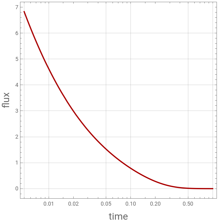
Plotting the mass flux versus time at x=1.
In[]:=
plt2=LogLinearPlot[Evaluate[D[c[x,t]/.sole,{x,1}]/.x1],{t,0.005,1},FrameTrue,AspectRatio1,GridLinesAutomatic,PlotStyle{Thick,Darker@Red},PlotRangeAll,PlotPoints1000,ImageSizeMedium,FrameLabel{Style["time",16],Style["flux",16]}]
Out[]=
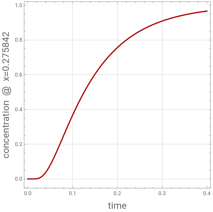
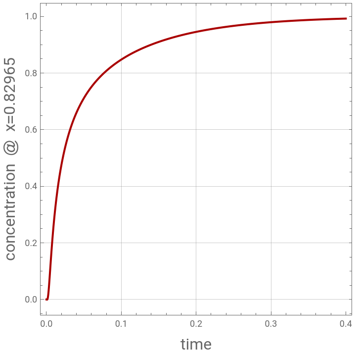
Plotting the concentrations versus time at x=0.829651 and x=0.275842.
In[]:=
plt3=Plot[c[x,t]/.sole/.x0.275842,{t,0,0.4},FrameTrue,AspectRatio1,GridLinesAutomatic,PlotStyle{Thick,Darker@Red},PlotRangeAll,PlotPoints1000,ImageSizeMedium,FrameLabel{Style["time",16],Style["concentration @ x=0.275842",16]}]
Out[]=
In[]:=
plt4=Plot[c[x,t]/.sole/.x0.82965,{t,0,0.4},FrameTrue,AspectRatio1,GridLinesAutomatic,PlotStyle{Thick,Darker@Red},PlotRangeAll,PlotPoints1000,ImageSizeMedium,FrameLabel{Style["time",16],Style["concentration @ x=0.82965",16]}]
Out[]=
Solution using Orthogonal Collocation
10 internal collocation points (N=10)
In[]:=
Np=10;
In[]:=
solj=SolveHypergeometric2F1-(Np),(Np)++1,,x^20,x;tbl=Select[Table[x/.solj[[i]],{i,1,Length[solj]}],#>0&];x[Np+1]=1.0;For[i=1,i<Np+1,{x[i]=tbl[[i]],i++}];
3.
2
3
2
In[]:=
TableForm@Table[x[i],{i,1,Np+1}]
Out[]//TableForm=
0.139276 |
0.275842 |
0.407038 |
0.530312 |
0.643264 |
0.743695 |
0.829651 |
0.899459 |
0.951758 |
0.985527 |
1. |
Matrix Q and
-1
Q
In[]:=
Q=Chop[Table[Table[x[j]^(2i-2),{i,1,11}],{j,1,11}]]
Out[]=
{{1.,0.0193979,0.000376277,7.29897×,1.41584×,2.74643×,0,0,0,0,0},{1.,0.0760886,0.00578947,0.000440512,0.000033518,2.55033×,1.94051×,1.47651×,1.12345×,0,0},{1.,0.16568,0.0274498,0.00454788,0.000753493,0.000124839,0.0000206832,3.4268×,5.67751×,9.4065×,1.55847×},{1.,0.281231,0.0790906,0.0222427,0.00625533,0.00175919,0.000494738,0.000139135,0.0000391291,0.0000110043,3.09475×},{1.,0.413788,0.171221,0.0708491,0.0293165,0.0121308,0.00501959,0.00207705,0.000859457,0.000355633,0.000147157},{1.,0.553082,0.3059,0.169188,0.0935748,0.0517546,0.0286245,0.0158317,0.00875625,0.00484293,0.00267854},{1.,0.688321,0.473786,0.326117,0.224473,0.154509,0.106352,0.0732043,0.0503881,0.0346832,0.0238732},{1.,0.809026,0.654523,0.529526,0.4284,0.346586,0.280397,0.226849,0.183526,0.148478,0.120122},{1.,0.905843,0.820552,0.743291,0.673305,0.609909,0.552482,0.500462,0.45334,0.410655,0.371989},{1.,0.971264,0.943353,0.916245,0.889915,0.864343,0.839505,0.815381,0.79195,0.769192,0.747088},{1.,1.,1.,1.,1.,1.,1.,1.,1.,1.,1.}}
-6
10
-7
10
-9
10
-6
10
-7
10
-8
10
-9
10
-6
10
-7
10
-8
10
-8
10
-6
10
In[]:=
IQ=Inverse[Q]
Out[]=
{{1.99026,-1.96094,1.9117,-1.84196,1.75069,-1.63625,1.49584,-1.32444,1.11198,-0.833339,0.336449},{-65.2434,139.599,-149.678,148.783,-143.404,135.024,-123.967,110.049,-92.5416,69.4145,-28.0351},{832.711,-2299.57,3126.96,-3354.21,3344.21,-3205.32,2973.29,-2656.,2241.96,-1685.26,681.219},{-5627.45,17617.,-27763.5,33007.5,-34625.,34119.,-32168.9,29024.,-24649.2,18592.2,-7525.64},{22806.4,-76764.5,132976.,-172208.,191542.,-195534.,188410.,-172322.,147586.,-111854.,45362.1},{-58867.4,207488.,-383194.,530168.,-622964.,661320.,-654024.,608427.,-526722.,401671.,-163302.},{99209.2,-360782.,697247.,-1.01502×,1.2509×,-1.38046×,1.40487×,-1.3331×,1.16916×,-898400.,366380.},{-108808.,404582.,-808438.,1.22443×,-1.57097×,1.79765×,-1.88405×,1.82745×,-1.62702×,1.2616×,-516419.},{74871.4,-283002.,579977.,-906324.,1.2028×,-1.42219×,1.53421×,-1.52303×,1.37901×,-1.08058×,444271.},{-29360.8,112372.,-234856.,376333.,-513814.,625522.,-693599.,705031.,-650117.,515529.,-213042.},{5006.68,-19349.,41072.8,-67172.5,93934.1,-117345.,133502.,-138930.,130601.,-104943.,43622.7}}
6
10
6
10
6
10
6
10
6
10
6
10
6
10
6
10
6
10
6
10
6
10
6
10
6
10
6
10
6
10
6
10
6
10
6
10
6
10
Matrix C
Matrix A
In[]:=
A=Ci.IQ
Matrix D
Matrix B
In[]:=
B=Di.IQ
Writing the system of ODEs to be solved
In[]:=
f[a_,b_]:=ab
In[]:=
eq=MapThread[f,{DC,B.Ce}]
Plotting the mass flux versus time at x=1.
Plotting the concentrations versus time at x=0.829651 and x=0.275842.
Comparing both solutions :
We get good agreement between the solution using NDSolve and the orthogonal collocation method.
In both cases, the mass flux is equal to 0.7842 at t=0.1 and x=1.
We get good agreement between the solution using NDSolve and the orthogonal collocation method.
In both cases, the mass flux is equal to 0.7842 at t=0.1 and x=1.