Introduction
Introduction
The number of ciphers that there are can make it difficult to even identify the type of one. Mathematica’s simple data visualization techniques, alongside its computational prowess, makes it a powerful tool for cryptographic analysis. By considering its potential for identification of more archaic ciphertext, it’s easy to see how it can both aid and automate processes of decryption for ciphers that are generally encrypted without a computer but can be extremely hard to decrypt by hand.
Exploration
Exploration
Simple encryption methods can be divided into two major categories: transposition and substitution ciphers. In the former characters are simply rearranged, whereas in the latter they are substituted with another. Transposition ciphers can generally be identified by considering how similar the frequencies of characters are in relation to those in a normal sentence in the language. For example, the letters E and T are generally the most common (especially due to their usage in words like ‘the’).
StringCount allows us to count the number of times a substring appears in a piece of data.
In[]:=
StringCount["The quick brown fox jumps over the lazy dog.","t"]
Out[]=
1
In ciphertext, capitals are generally without purpose, so it is best to convert it into lower case (or upper case: either way removes issues) to prevent any problems in parsing data.
In[]:=
StringCount[ToLowerCase["The quick brown fox jumps over the lazy dog."],"t"]
Out[]=
2
A For loop allows us to iterate over this to get the frequencies for every letter. The Alphabet can be changed for each language.
In[]:=
alphabet=Alphabet[];
data=ToLowerCase["The quick brown fox jumps over the lazy dog."];frequencies={};For[i=1,i<Length[alphabet]+1,i++,AppendTo[frequencies,StringCount[data,alphabet[[i]]]]]Print[frequencies]
{1,1,1,1,3,1,1,2,1,1,1,1,1,1,4,1,1,2,1,2,2,1,1,1,1,1}
We can then plot the frequencies in a bar chart, like so:
In[]:=
BarChart[frequencies,ChartLabels->alphabet]
Out[]=
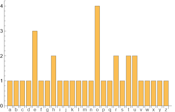
For large pieces of text (and of course, those that aren’t a pangram), we’d expect to see more variation . Let’s consider the first passage from H.G. Well’s The War of the Worlds.
In[]:=
newdata=ToLowerCase["No one would have believed, in the last years of the nineteenth century, that human affairs were being watched keenly and closely by intelligences greater than man's and yet as mortal as his own; that as men busied themselves about their affairs they were scrutinised and studied, perhaps almost as narrowly as a man with a microscope might scrutinise the transient creatures that swarm and multiply in a drop of water. With infinite complacency men went to and fro over this globe about their little affairs, serene in their assurance of their empire over matter. It is possible that the infusoria under the microscope do the same. No one gave a thought to the older worlds of space as sources of human danger, or thought of them only to dismiss the idea of life upon them as impossible or improbable. It is curious to recall some of the mental habits of those departed days. At most, terrestrial men fancied there might be other men upon Mars, perhaps inferior to themselves and yet ready to welcome a missionary enterprise. Yet, across the gulf of space, minds that are to our minds as ours are to those of the beasts that perish, intellects vast and cool and unsympathetic, regarded this earth with envious eyes, and slowly and surely drew their plans against us."];passagefrequencies={};For[i=1,i<Length[alphabet]+1,i++,AppendTo[passagefrequencies,StringCount[newdata,alphabet[[i]]]]];BarChart[passagefrequencies,ChartLabels->alphabet]
Out[]=
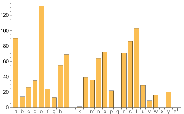
With that, even itself being only a small piece, we see a more satisfying response. E holds the top spot, with T soon after. There is a large amount of variation which is what we should expect to see within a transposition cipher. If, however, we consider that with something like the Vigenère (a keyed substitution cipher), we’ll see much different results. Using the same text and keyword ‘wells’:
In[]:=
vigdata=ToLowerCase["Js zyw ssfwv degp taptpnah, ty ldi wlkp cpljo sq eza rtywpipyld gpylqvj, ezwx sfewr lqxwmcd oavp mwerr hspgspv gipydu eyo uhsdpdu fj tfpiwwaciynwo kcpspic ezwr xlf'o eyo qax ld ekveld ww stk kay; ezwx ld ear mfkeio ezaqdpdrid ltkye ezamc lxbetck plpj oavp dunyetfewpo sjh demzmpo, havslho ewxgox ld fwvczohc ld s iey hapl l xayvzduktp xacle dunyetfewp eza xclfompyl yvpllqvpd ldee dowvx lfz qfwletwj aj e ocgl sq hspic. Hapl tyxertew ysxadwgpyuu qpy oare eg wro qjk sgpj pltd yhsmp sxsfe lditc dexeww wjqlanw, dpjarp tf plptj wwdfjwrnp gb xspan ixaani zgwn qlelav. Te ao tzdkefwp ldee eza myqmoscts qropj plp xayvzduktp og plp dsii. Yz gji rlna e esgqkse lk xsp ghhpc okvwok kj dasyi ld kkycnwo sq smiey osjkpc, gn xszmcle zx plpx gjpj eg zmdxaow esw ehpl gb ptqw qtzy ldix lk eqazkommww kv txhnsmlthi. Te ao gfcakyd eg ninldh wzxw kj esw iiyesh llmapw zq ldsdp vatlclah olqo. Ee xgox, epjnidejeew xwj jlyueio ezavp xacle mw kxspj iiy fhkr Xljo, tpczwtd tfbictgn xz ezaqdpdrid lfz cpe jaeoj lk apwukqp l eewdtgjecj wjxpchnmdp. Qax, lnjkwd eza kfwx kj dasyi, xtfzw essp ecp lk sfc eerod so sfck wvp eg plzdw kj esw xildlo xsll lictkd, myewhppnlo zldl wro ngkp lyv qrdjeleeswpmn, cwcecowz xstk aecez smes wjztzmo ijpk, wro ddkawj sjh dfjapj ojaa eswev awsjw lrserde mo."];newpassagefrequencies={};For[i=1,i<Length[alphabet]+1,i++,AppendTo[newpassagefrequencies,StringCount[vigdata,alphabet[[i]]]]];BarChart[newpassagefrequencies,ChartLabels->alphabet]
Out[]=
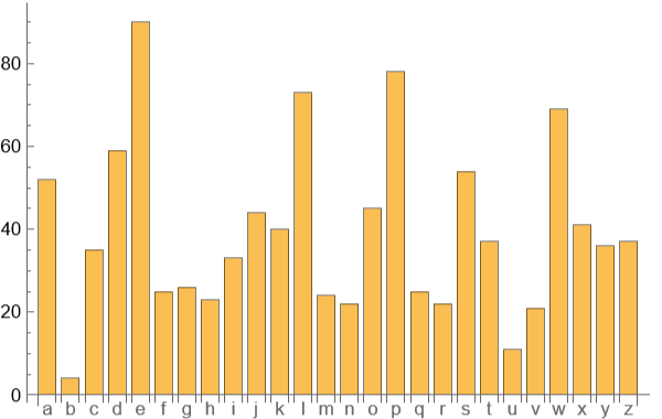
With that we still see some variation, but much less. Whereas we missed some letters completely in the passage before, now there is a larger number of every letter. While E is still with the highest frequency, the others are not what we’d expect to see, with letters like Z and Y being extremely high. Generally this allows us to distinguish between Transposition and Substitution ciphers. This is where something like Mathematica is very helpful, because of the easy and quick data visualization.
Going further in, we can distinguish more between substitution ciphers, even going so far as being able to decrypt them completely (whereas transposition ciphers are hard to decrypt without complex consideration, due to the sheer number of permutations needed). The Affine and Caesar shift ciphers are simple, and can be brute-forced. They shift the letters a certain number of places, for example A->B, B->C. The Affine cipher does this by multiplying rather than adding, but even this only has around 312 possible types of shift, so can also easily be decrypted. We won’t delve into that. If you were to consider a graph of the same passage but done with one of these ciphers, you’d actually see a graph more similar to the first, with more variation. However you’d also see a change of common frequencies, like N being the most common letter. This is a common method of decrypting a cipher without brute force:
the most common letters are identified, and then formulae for the shifts that would move E to that letter are calculated (E being the most common, generally).
In considering whether a graph is more varied therefore, it’s quite easy also to see whether or not the ciphertext uses something more complex. These are called poly-alphabetic ciphers, as depending on the key and method the same letter is encoded into something different. We’ll delve into the Vigenère, as there are so many ciphers that it would be impossible to cover them all.
Such a cipher would have a graph similar to the one shown up above, with quite a large frequency for each letter. The main weak point of ciphers like these is that the key will be repeating all the time. So if we have a 7 letter long keyword, the 1st letter and the 8th letter of the ciphertext will have been encrypted by the same monoalphabetic cipher. So, let’s say that we know the key is 7 letters long. For each set of letters that belong to the same monoalphabetic cipher, we can then use frequency analysis to estimate what actual letter it is bound too, and effectively reverse engineer the cipher for each character of the keyword.
For a cipher that we don’t know the key, we’ll have to try and find the key length and do the same. Obviously this would take too long by hand, but luckily there’s a fantastic technique that we can use to help us: the Index of Coincidence. We run the calculation to find, effectively, a probability, and by the end we have a decimal result. If the result is around 0.0667, it’s likely English. We’ll start by using the same code to get the frequencies of each letter.
In[]:=
alphabet=Alphabet[];iocdata=ToLowerCase["No one would have believed, in the last years of the nineteenth century, that human affairs were being watched keenly and closely by intelligences greater than man's and yet as mortal as his own; that as men busied themselves about their affairs they were scrutinised and studied, perhaps almost as narrowly as a man with a microscope might scrutinise the transient creatures that swarm and multiply in a drop of water. With infinite complacency men went to and fro over this globe about their little affairs, serene in their assurance of their empire over matter. It is possible that the infusoria under the microscope do the same. No one gave a thought to the older worlds of space as sources of human danger, or thought of them only to dismiss the idea of life upon them as impossible or improbable. It is curious to recall some of the mental habits of those departed days. At most, terrestrial men fancied there might be other men upon Mars, perhaps inferior to themselves and yet ready to welcome a missionary enterprise. Yet, across the gulf of space, minds that are to our minds as ours are to those of the beasts that perish, intellects vast and cool and unsympathetic, regarded this earth with envious eyes, and slowly and surely drew their plans against us."];iocfrequencies={};For[i=1,i<Length[alphabet]+1,i++,AppendTo[iocfrequencies,StringCount[iocdata,alphabet[[i]]]]];Print[iocfrequencies]
{90,14,26,35,132,24,13,55,69,0,1,39,36,64,72,22,0,71,86,103,29,9,16,0,20,0}
IOC calculation (removing all non-alphabet characters)
ioclength=StringLength[StringReplace[iocdata,Except[LetterCharacter]->""]];total=0;For[j=1,j<=Length[iocfrequencies],j++,total=total+(iocfrequencies[[j]]*(iocfrequencies[[j]]-1))];ioc=N[total/(ioclength*(ioclength-1))]
72332
Out[]=
0.0687795
That gives us a beautifully aligned result, showing us that it’s in plain English. Now, were we to separate our ciphertext into the characters that would be encoded by the same letter for each key length (say, up to 9), we’d see an index of coincidence closest to around that value for the proper key length. When we split it up of course, we’ll get several sets of letters, so we can get a mean index of coincidence for more accuracy: to keep things simple though, we’ll just consider the first letters matching a key length.
In[]:=
index[tdata_]:=(data=ToLowerCase[tdata];iocfrequencies={};For[i=1,i<Length[alphabet]+1,i++,AppendTo[iocfrequencies,StringCount[data,alphabet[[i]]]]];ioclength=StringLength[StringReplace[data,Except[LetterCharacter]->""]];total=0;For[j=1,j<=Length[iocfrequencies],j++,total=total+(iocfrequencies[[j]]*(iocfrequencies[[j]]-1))];ioc=N[total/(ioclength*(ioclength-1))];Return[ioc])split[data_,splitting_]:=(x=Partition[Characters[data],splitting];returning={};For[i=1,i<=Length[x],i++,AppendTo[returning,x[[i]][[1]]]];Return[StringJoin[returning]])encodeddata=StringReplace[ToLowerCase["Js zyw ssfwv degp taptpnah, ty ldi wlkp cpljo sq eza rtywpipyld gpylqvj, ezwx sfewr lqxwmcd oavp mwerr hspgspv gipydu eyo uhsdpdu fj tfpiwwaciynwo kcpspic ezwr xlf'o eyo qax ld ekveld ww stk kay; ezwx ld ear mfkeio ezaqdpdrid ltkye ezamc lxbetck plpj oavp dunyetfewpo sjh demzmpo, havslho ewxgox ld fwvczohc ld s iey hapl l xayvzduktp xacle dunyetfewp eza xclfompyl yvpllqvpd ldee dowvx lfz qfwletwj aj e ocgl sq hspic. Hapl tyxertew ysxadwgpyuu qpy oare eg wro qjk sgpj pltd yhsmp sxsfe lditc dexeww wjqlanw, dpjarp tf plptj wwdfjwrnp gb xspan ixaani zgwn qlelav. Te ao tzdkefwp ldee eza myqmoscts qropj plp xayvzduktp og plp dsii. Yz gji rlna e esgqkse lk xsp ghhpc okvwok kj dasyi ld kkycnwo sq smiey osjkpc, gn xszmcle zx plpx gjpj eg zmdxaow esw ehpl gb ptqw qtzy ldix lk eqazkommww kv txhnsmlthi. Te ao gfcakyd eg ninldh wzxw kj esw iiyesh llmapw zq ldsdp vatlclah olqo. Ee xgox, epjnidejeew xwj jlyueio ezavp xacle mw kxspj iiy fhkr Xljo, tpczwtd tfbictgn xz ezaqdpdrid lfz cpe jaeoj lk apwukqp l eewdtgjecj wjxpchnmdp. Qax, lnjkwd eza kfwx kj dasyi, xtfzw essp ecp lk sfc eerod so sfck wvp eg plzdw kj esw xildlo xsll lictkd, myewhppnlo zldl wro ngkp lyv qrdjeleeswpmn, cwcecowz xstk aecez smes wjztzmo ijpk, wro ddkawj sjh dfjapj ojaa eswev awsjw lrserde mo."],Except[LetterCharacter]->""];iocs={};For[a=2,a<=9,a++,AppendTo[iocs,index[split[encodeddata,a]]]];Print[iocs]
Representing in a bar chart and comparing to an expected IOC.
And as seen, our closest keyword that has an IOC close to a proper one is that with length 5: which, if you remember is correct, as our keyword is ‘wells’. From there it’s a simple matter to decode it! This proves that it is a Vigenère, too, or at least some sort of similar cipher.
These simple techniques are easy to implement but provide a strong toolkit for cryptographic analysis of simple ciphers. Wolfram also has a large number of functions for ciphers that may be computer-generated, like asymmetric encryption, but exploring ciphers like these can provide a good foundation going into more advanced cryptanalysis.