ABSTRACT (original article): The present paper describes the arc-length continuation method; a mathematical technique that can solve a wide variety of chemical engineering problems. Several case studies involving distillation, reaction engineering, and thermodynamics are treated with the help of this method. The approach is powerful enough to elucidate situations when several turning points occur. Finally, the authors conclude with their experience teaching this technique. Indeed, this methodology was introduced to the graduate students of the nonlinear dynamics course at King Fahd University of Petroleum & Minerals (KFUPM). CITATION (original article): Binous, H., & Shaikh, A. A. (2014). Introduction of the arc-length continuation technique in the chemical engineering graduate program at KFUPM. In Computer Applications in Engineering Education. DOI: https://doi.org/10.1002/cae.21604
The figure shows a bifurcation-style diagram obtained for a binary ethanol-water batch rectification column, where the reflux ratio (R) is used as the continuation parameter and the distillate composition (xD) is the response variable.Two independent continuation strategies are implemented:1. Predictor-corrector arc-length continuation using FindRoot2. Differential-algebraic continuation using NDSolveBoth methods generate the same solution branch, confirming the numerical consistency of the continuation procedure.The vapor-liquid equilibrium (VLE) behavior is modeled using the Van Laar activity coefficient model together with Antoine vapor pressure correlations. The equilibrium relation is obtained from modified Raoult’s law: where are the activity coefficients computed from the Van Laar equations. The resulting nonlinear equilibrium curve is interpolated and used inside the stage equations of the rectifying section.The rectifying operating line is written as which couples the tray liquid compositions, vapor compositions, reflux ratio, and distillate composition.Although batch rectification is fundamentally a dynamic process, the column hydraulics and tray mass-transfer dynamics are usually much faster than the slow depletion of material in the reboiler. For this reason, the column is approximated as operating under a sequence of steady states. At every instant, the internal tray profiles are assumed to rapidly equilibrate relative to the slow variation of the still composition. This approximation is called the pseudo-steady-state assumption.Under this assumption:• Tray vapor-liquid equilibrium relations remain algebraic• The operating line is valid instantaneously• The dynamic evolution is represented indirectly through the continuation parameter (R)As the reflux ratio changes, the column moves continuously through a family of steady operating states. Arc-length continuation is therefore an efficient tool for tracing the complete solution branch without explicitly integrating transient mass balances.The first approach uses a classical arc-length continuation algorithm. Starting from a converged solution at (R = 0.5), a tangent vector is estimated and a predictor step is performed along the solution branch. The continuation constraint is : where:• z is the augmented variable vector• is the predicted point• t is the tangent vectorA Newton corrector (FindRoot) then solves the augmented nonlinear system composed of:• stage equilibrium equations,• operating line equations,• boundary conditions,• arc-length constraint.
P=
y
i
γ
i
x
i
sat
P
i
γ
i
y=x+
R
R+1
xD
R+1
(z-)·t=0
z
pred
z
pred
This method is robust because it can follow highly nonlinear solution branches even near turning points where ordinary parameter continuation may fail.The second strategy (decribed thoroughly in Ref. 1) reformulates the continuation problem as a differential-algebraic system parameterized by the arc-length variable (s). The continuation equations are supplemented by a normalization condition: +=1.
2*Ns+1
∑
i=1
2
u
i
s
2
R
s
This equation enforces unit arc-length parametrization and allows Mathematica’s NDSolve to integrate directly along the solution branch.
The method behaves like geometric continuation in an extended state space and avoids repeated external predictor-corrector loops.
The resulting diagram shows that increasing the reflux ratio improves the distillate purity. At low reflux ratios, the separation efficiency is limited and the distillate ethanol composition remains relatively low. As the reflux ratio increases, the operating line approaches the equilibrium curve, leading to improved separation and higher distillate purity.
However, the curve progressively flattens at high reflux ratios, indicating diminishing returns: increasingly large reflux ratios produce only small improvements in purity. This is a classical behavior in distillation design and reflects the thermodynamic limitations imposed by vapor-liquid equilibrium.
The overlap between the red solid curve (predictor-corrector continuation) and the blue dashed curve (DAE continuation) demonstrates that both continuation formulations trace the same nonlinear solution manifold accurately.
In[]:=
ClearAll["Global`*"]
Antoine Equation where Temperature in °C and Pressure in mmHg
Ethanol
Psat1[T_]:=10^(8.20417-1642.89/(230.3+T));
Water
Psat2[T_]:=10^(8.07131-1730.63/(233.426+T));
Normal boiling temperatures
In[]:=
FindRoot[Psat1[T]==760,{T,80}]FindRoot[Psat2[T]==760,{T,80}]
Out[]=
{T78.3192}
Out[]=
{T99.9968}
Van Laar Model
gamma1[x_]:=Exp[A12(A21(1-x)/(A12x+A21(1-x)))^2];gamma2[x_]:=Exp[A21(A12x/(A12x+A21(1-x)))^2];A12=1.6798;A21=0.9227;(*binaryinteractionparameters*)
In[]:=
Ptot=760;
In[]:=
i=1;While[i<=101,{xe[i]=(i-1)0.01,sol[i]=Quiet@FindRoot[{xe[i]gamma1[xe[i]]Psat1[T]+(1-xe[i])gamma2[xe[i]]Psat2[T]==Ptot},{T,95}],ye[i]=xe[i]gamma1[xe[i]]Psat1[T]/Ptot/.sol[i],i++}];
In[]:=
vle=Interpolation[Table[{xe[i],ye[i]},{i,1,101}]]
Out[]=
InterpolatingFunction


In[]:=
Plot[vle[x],{x,0,1},Frame->True,GridLines->Automatic,AspectRatio->1,FrameLabel->{Style[x,14],Style[y,14]},Epilog->{Green,Thickness[0.0025],Line[{{0,0},{1,1}}]}]
Out[]=
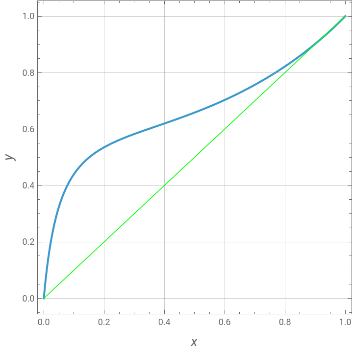
Azeotropic composition
FindRoot[vle[x]==x,{x,0.85}]
Out[]=
{x0.91489}
Still composition
xB=0.40;
Number of rectifying stages
Nstage=15;
Continuation parameters
ds=0.5;nSteps=2000;
VLE equation for Ethanol-Water mixture
yEq[x_]:=vle[x]
Rectifying operating line
yOp[x_,xD_,R_]:=(R/(R+1))*x+xD/(R+1)
Stage equations
stageEquations[vars_,R_]:=Module[{x,y,xD,eqs},x=vars[[1;;Nstage]];y=vars[[Nstage+1;;2Nstage]];xD=vars[[-1]];eqs={};(*equilibriumrelations*)Do[AppendTo[eqs,y[[i]]==yEq[x[[i]]]],{i,1,Nstage}];(*operatinglinerelations*)Do[AppendTo[eqs,y[[i]]==yOp[x[[i+1]],xD,R]],{i,1,Nstage-1}];(*condenser*)AppendTo[eqs,y[[Nstage]]==xD];(*reboilerboundary*)AppendTo[eqs,x[[1]]==xB];eqs]
Variables
vars=Join[Table[x[i],{i,Nstage}],Table[y[i],{i,Nstage}],{xD}];
Initial solution at reflux ration R=1
R0=0.5;guess=Join[Table[0.4,{i,Nstage}],Table[0.9,{i,Nstage}],{0.85}];sol0=FindRoot[stageEquations[vars,R0],Evaluate@Thread[{vars,guess}],MaxIterations->100];u0=vars/.sol0;Print["Initial Distillate Composition = ",xD/.sol0];
First Method based on FindRoot and predictor / corrector scheme
Bifurcation diagram
Second Method, thoroughly described in Ref. 1, is based on NDSolve and solving a system of DAEs
References
References
[1] Binous, H., & Shaikh, A. A. (2014). Introduction of the arc-length continuation technique in the chemical engineering graduate program at KFUPM. In Computer Applications in Engineering Education (Vol. 23, Issue 3, pp. 344–351). Wiley. DOI: https://doi.org/10.1002/cae.21604
CITE THIS NOTEBOOK
CITE THIS NOTEBOOK
Batch rectification of ethanol-water mixture by arc-length continuation
by Housam Binous and Abdullah Shaikh
Wolfram Community, STAFF PICKS, May 27, 2026
https://community.wolfram.com/groups/-/m/t/3723119
by Housam Binous and Abdullah Shaikh
Wolfram Community, STAFF PICKS, May 27, 2026
https://community.wolfram.com/groups/-/m/t/3723119