The Hodgkin-Huxley model is a cornerstone of computational neuroscience, providing a mathematical description of how action potentials in neurons are initiated and propagated. It was formulated by Alan Lloyd Hodgkin and Andrew Fielding Huxley in 1952, for which they were awarded the Nobel Prize in Physiology or Medicine in 1963. This model describes how electrical characteristics of the cell membrane evolve over time in response to stimuli, using a set of nonlinear differential equations.
Model Overview
Model Overview
The Hodgkin-Huxley model accounts for the dynamics of the membrane potential by considering the flow of sodium (Na+), potassium (K+), and leak currents through specific ion channels. The conductances of these ion channels are not constant but vary with both the membrane potential and time, leading to the complex behavior of action potentials.
Implementation in Mathematica
Implementation in Mathematica
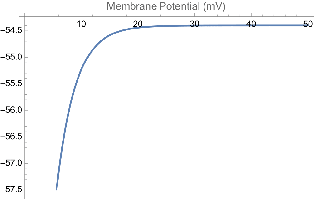
In this example, we implement the Hodgkin-Huxley model in Mathematica. We define the model parameters, equations, and initial conditions, and then solve the equations using `NDSolve`. Finally, we plot the membrane potential over time to visualize the action potential.
Model Parameters
Model Parameters
The parameters represent the conductances for sodium (\(g_{Na}\)), potassium (\(g_K\)), and leak (\(g_L\)) channels, their respective Nernst potentials (\(E_{Na}\), \(E_K\), \(E_L\)), and the membrane capacitance (\(C_m\)).
(*Hodgkin-HuxleyModelParameters*)gNa=120;(*Sodiumconductance*)gK=36;(*Potassiumconductance*)gL=0.3;(*Leakconductance*)ENa=50;(*SodiumNernstpotential*)EK=-77;(*PotassiumNernstpotential*)EL=-54.4;(*LeakNernstpotential*)Cm=1;(*Membranecapacitance*)
Hodgkin-Huxley Equations
Hodgkin-Huxley Equations
The model’s core consists of four differential equations describing the evolution of the membrane potential (\(V\)) and the gating variables (\(m\), \(h\), \(n\)).
Hodgkin-Huxley Model Equations
eqns={CmV'[t]==gNam[t]^3h[t](ENa-V[t])+gKn[t]^4(EK-V[t])+gL(EL-V[t]),m'[t]==alphaM[V[t]](1-m[t])-betaM[V[t]]m[t],h'[t]==alphaH[V[t]](1-h[t])-betaH[V[t]]h[t],n'[t]==alphaN[V[t]](1-n[t])-betaN[V[t]]n[t]};
Alpha and Beta Functions
Alpha and Beta Functions
These functions describe the voltage-dependent rates at which the gating variables change.
Alpha and Beta Functions
alphaM[v_]:=0.1(25-v)/(Exp[(25-v)/10]-1);betaM[v_]:=4Exp[-v/18];alphaH[v_]:=0.07Exp[-v/20];betaH[v_]:=1/(Exp[(30-v)/10]+1);alphaN[v_]:=0.01(10-v)/(Exp[(10-v)/10]-1);betaN[v_]:=0.125Exp[-v/80];
Solving and Plotting
Solving and Plotting
We solve the equations with initial conditions close to a resting state and plot the membrane potential over time.
Initial Conditions and Time Span
initialConditions={V[0]==-65,m[0]==0.05,h[0]==0.6,n[0]==0.32};timeSpan={t,0,50};
Solve the Equations
sol=NDSolve[Join[eqns,initialConditions],{V,m,h,n},timeSpan];
Plot the Results
Plot[Evaluate[V[t]/.sol],{t,0,50},PlotLabel->"Membrane Potential (mV)"]
Conclusion
Conclusion
The Hodgkin-Huxley model provides deep insights into the biophysical mechanisms underlying nerve excitability. This Mathematica implementation offers a concise and powerful way to explore and visualize the dynamics of neuronal action potentials. It serves as a foundational tool for further exploration in computational neuroscience and beyond.
CITE THIS NOTEBOOK
CITE THIS NOTEBOOK
Simulating Neuronal Dynamics with the Hodgkin-Huxley Model in Mathematica
by Srujan Yamali
Wolfram Community, STAFF PICKS, February 14, 2024
https://community.wolfram.com/groups/-/m/t/3122270
by Srujan Yamali
Wolfram Community, STAFF PICKS, February 14, 2024
https://community.wolfram.com/groups/-/m/t/3122270