Intro
Intro
In the previous post, we tried to classify stable centroidal Voronoi tessellations and encountered typical problems of selecting criteria and methods for decision-making. Also left unaddressed unstable CVT. We can get more detailed and informative answers if you we the s.c. energy approach. Moreover, it is a good and profound illustration of such difficult concepts as the hessian, saddle points etc. in multidimensional spaces.
General utilities
General utilities
In[]:=
Clear[arrDistC,lloydStepOrdered,lloydProc,lloydProcList,voronPlot];(*Distancebetweenarraysofpoints*)arrDistC=Block{nf},Compile{{arr1,_Real,2},{arr2,_Real,2}}, (nf=Nearest@arr1;Total[EuclideanDistance[First@nf@#,#]&/@arr2]);(*MainLloydstepwithorderingcells*)lloydStepOrdered[pts_]:=Block[{m={VoronoiMesh[pts,{{0,1},{0,1}}],2}},AnnotationValue[m,MeshCellCentroid][[NearestMeshCells[m,#][[1,2]]&/@pts]]];(*Lloydprocess*)lloydProc[pts_,tol_,maxIt_]:=NestWhile[lloydStepOrdered@#&,pts,arrDistC@##>tol&,2,maxIt];lloydProcList[pts_,maxIt_]:=NestList[lloydStepOrdered@#&,pts,maxIt];(*Graphics*)voronPlot[pts_,size_:70]:=With{mesh=VoronoiMesh[pts,{{0,1},{0,1}}]},GraphicsEdgeForm@Black,FaceForm@DarkGray,mesh, StandardOrange,PointSize@.06,Point@pts,ImageSizesize;
Main definitions
Main definitions
Energy
Energy
For seeds and cells Voronoi tessellation energy function is:
s
i
Ω
i
Ε
i
s
i
∫
Ω
i
2
-
r
s
i
r
∑
i
Ε
i
⋆ Pattern is centroidal if that is critical point of Ε (zeroes of gradient).
s
i
⋆ CVT is a stable CVT if it is a local minimizer of Ε()
s
i
⋆ It is called an optimal CVT if it is a global minimizer of Ε()
s
i
⋆ Saddle points of Ε() are unstable CVT.
s
i
It had shown that the energy E has second order smoothness for convex domains, therefore we can apply classical optimization methods: Newton, Nelder-Mead etc. By playing a little with integrals, we can get expressions for energy and gradient, which are calculated fairly quickly is centroid of i-th cell):
(isareaand
a
i
c
i
Ε=+-2·where=-secondmoment=2-
s
i
∑
i
Ι
i
a
i
2
s
i
a
i
s
i
c
i
Ι
i
∫
Ω
i
2
r
r
Γ
s
i
∑
i
a
i
s
i
c
i
In the process of generating VoronoiMesh we already get areas and centroids; and tests show that their extraction with AnnotationValue is as fast as arithmetic calculation. Now, the moment of inertia is better calculated directly. Although I might be told how to compile MomentOfInertia for convex polygon for quick work.
Hessian
Hessian
Hessian is a square matrix of second-order partial derivatives of a scalar-valued function (Voronoi energy in this post). It is important to understand that in our case all coordinates must be flatten and the indices j, k run through values 1.. 2N:
Η
jk
s
2
∂
∂∂
v
j
v
k
v
1
s
1x
v
2
s
1y
v
2N
s
Ny
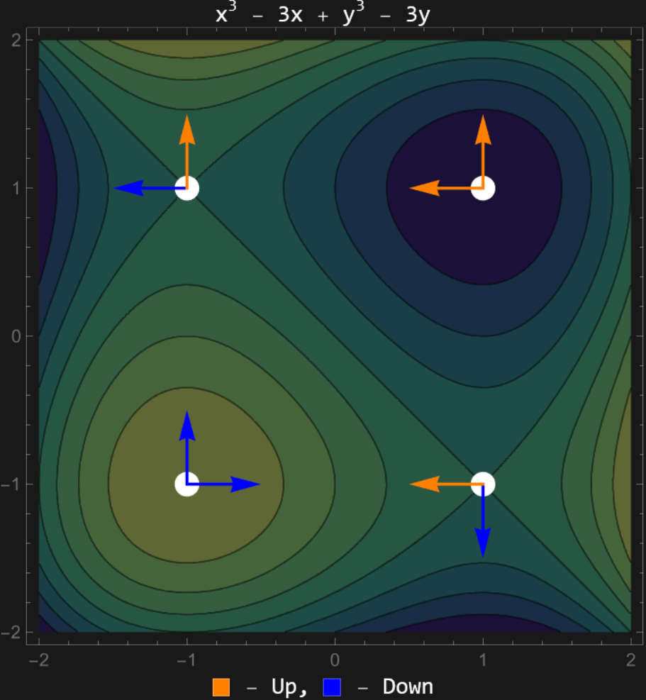
As we "go" from the critical point in some direction, we will go either "up" - the function will increase, or downward - to decrease. For the maximum, we go down in any direction; for the minimum, we go up. From saddle points, some paths lead up, others down. Eigenvectors of hessian show directions of fastest descent/ascent, a signs of eigenvalues - the "slope" direction. For a two-dimensional case, it is easy to visualize:
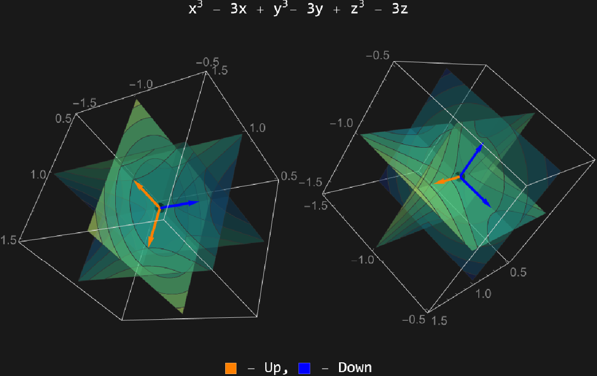
In multidimensional saddle point cases, there can be different numbers of "up" and "down" directions:
Unfortunately, the exact formulas for Hessian of Voronoi energy are complex and not simplified.
But we need only qualitative assessments, so let’s use simple numerical approximation:
But we need only qualitative assessments, so let’s use simple numerical approximation:
Η
jk
Γ
j
v
1
v
k
v
2N
Γ
j
v
1
v
k
v
2N
2h
v
1
s
1x
v
2
s
1y
v
2N
s
Ny
The most important characteristic of hessian is signature σ(Η) - total of signs of eigenvalues.
Main functions
Main functions
Clear[momentC,momentP,helperEV,energyV,gradV,gradVFlat,hessV,hessSgn];(*Compiledcoreofinertiamoment*)momentC=Compile{{xx,_Real,1},{yy,_Real,1},{n,_Integer}},Sum[(xx[[k]]*yy[[k+1]]-xx[[k+1]]*yy[[k]])*(+xx[[k+1]]*xx[[k]]+++yy[[k]]*yy[[k+1]]+),{k,n-1}]+(xx[[n]]*yy[[1]]-xx[[1]]*yy[[n]])*(+xx[[1]]*xx[[n]]+++yy[[n]]*yy[[1]]+);(*Momentofinertiaforpolygon*)momentP[poly_]:=Block[{xx,yy},{xx,yy}=Transpose@First@poly;momentC[xx,yy,Length@xx]/12.];helperEV=Compile[{{p,_Real,1},{c,_Real,1},{a,_Real},{m,_Real}},m+a*p.p-2.*a*p.c];(*Voronoitessellationenergyfunction*)energyV[pts_]:=With[{mesh=VoronoiMesh[pts,{{0,1},{0,1}}]},{ord=NearestMeshCells[mesh,#][[1,2]]&/@pts},{moments=momentP/@MeshPrimitives[mesh,2][[ord]]},{areas=AnnotationValue[{mesh,2},MeshCellMeasure][[ord]]},{cnts=AnnotationValue[{mesh,2},MeshCellCentroid][[ord]]},Total@MapThread[helperEV@##&,{pts,cnts,areas,moments}]]/;MatrixQ[pts,NumericQ];(*Energygradientastensor*)gradV[pts_]:=With[{mesh=VoronoiMesh[pts,{{0,1},{0,1}}]},{ord=NearestMeshCells[mesh,#][[1,2]]&/@pts},{areas=AnnotationValue[{mesh,2},MeshCellMeasure][[ord]]},{cnts=AnnotationValue[{mesh,2},MeshCellCentroid][[ord]]},MapThread[2#3(#1-#2)&,{pts,cnts,areas}]]/;MatrixQ[pts,NumericQ];(*Flattenedgradient*)gradVFlat[pts_]:=Flatten@gradV@pts/;MatrixQ[pts,NumericQ];(*Symmertrizedhessianastensor*)hessV[pts_]:=Block[{num=Length@pts,ptsF=Flatten@pts,h=0.01},Table[.5(gradVFlat[Partition[ptsF+hUnitVector[2num,j],2]][[i]]-gradVFlat[Partition[ptsF-hUnitVector[2num,j],2]][[i]])/h,{i,2num},{j,2num}]];(*Totalsignatureofhessianeigenvaluesσ(h)*)hessSgn[pts_]:=Total@Sign[Eigenvalues@hessV@pts];
2
xx[[k+1]]
2
xx[[k]]
2
yy[[k+1]]
2
yy[[k]]
2
xx[[1]]
2
xx[[n]]
2
yy[[1]]
2
yy[[n]]
Energy optimization - stable CVT
Energy optimization - stable CVT
This module finds a local minimum of energy near the initial configuration init.
Example for 7 seeds:
The result is very similar to that obtained with Lloyd’s algorythm in the previous post. Energy optimization works even slower, especially with large N’s. But now we can answer the question "Which configuration is better?"
For a small number of centers, all possible SCVTs equivalent to dihedral group turns and reflections can be found and distinguished. It may be a “childhood” question - which one is the “best of all”?
There are two important observations here:
2. As we have seen, at N = 7 the local minima differ by 1.2%. When increasing N, this difference becomes even smaller and ultimately the objective of global optimization becomes so flat that it is poorly solved even by special algorithms.
Unstable CVT
Unstable CVT
But the energy approach allows us to advance into such a little-explored field, as unstable CVT search and analysis. As stated, UCVT are saddle points of energy function. Neither Lloyd process nor energy optimization finds these configurations. Mathematically saddle point is a point where:
⋆ Gradient has a root
⋆ Hessian has at least one negative eigenvalue
There are algorithms, similar to Newton’s, that convergence exactly to saddle points. Due to the multidimensionality and non-convex relief, implementing such an algorithm for energy function of CVT is difficult. However, we will suggest an approach that allows this to be done with Mathematica. At the beginning, we will conduct some general research.
How really unstable?
How really unstable?
Consider the following (intuitively found) UCVT for 3 seeds configurations:
For each of them, we will fix two seeds and construct energy contours for the free seed on a square basis. In each case, we will have two fundamentally different configurations:
We see classic relief with all kinds of extreme points: maxima, minima and saddle points. The nature of saddle points, however, differs in each configuration, as indicated by σ. In fact, unstable CVTs are not totally unstable. Let’s do an experiment like this. We’ll move some seed in a little step, moving in a certain direction. After each step, we will run the Lloyd process and see what happens to the configuration. Different configurations and directions will produce different characteristic results.
We see all possible results of the relaxation process behavior near the saddle point:
1. Even slightest deviation leads to a shift from saddle point to the nearest energy minimum
2. With small deviations, the system returns back; with large ones, it runs to a minimum.
3. Even with significant deviations saddle point shows stability.
Hessian signature behavior in Lloyd process
Hessian signature behavior in Lloyd process
If a random set of N seeds is selected, then the Voronoi energy' hessian is likely to have a small signature - approximately the same numbers of directions in which the energy decreases or increases.
Interesting to see how the signature changes when conducting the Lloyd process:
We can see that the LLoyd process behaves in a non-trivial way. Sometimes it immediately reaches a minimum (where σ = 2 N. But sometimes it hangs out in the saddles for a long time, and even returns to more unstable states!
Interestingly also, what is the statistic of the number of steps needed to get to the area where σ = 2 N? I have not encountered such research. Next cell needs~3min to get result.
Collecting unstable CVT
Collecting unstable CVT
We now have everything needed for a targeted UCVT search. Observation of signature behavior in Lloyd process shows that one can start with a random set of seeds and perform a few steps of this algorithm, monitoring the signature. If it doesn’t get too big, then we’re closer to the saddle point and can look for root of gradient. Best suited for this is FindRoot with "Secant" method.
Example of usage:
Using this module we can collect all (?) CVT for N = 3
Transitions between patterns
Transitions between patterns
As we have seen above, with small deviations from the SCVT, energy increases in any direction. So when Lloyd is launched, they will come back.
But if the deviation is large enough, there may be switch to the neighboring SCVT. The same is true for UCVT. Transitions can also occur as jump of gradient zero. We can construct transition graphs between all CVTs for different values of deviation from the original state. The transitions in the LLoyd relaxation process are indicated by blue, while red is the result of finding gradient zeroes.
But if the deviation is large enough, there may be switch to the neighboring SCVT. The same is true for UCVT. Transitions can also occur as jump of gradient zero. We can construct transition graphs between all CVTs for different values of deviation from the original state. The transitions in the LLoyd relaxation process are indicated by blue, while red is the result of finding gradient zeroes.
For δ = 0.02, the situation is clear: there will always be a deflection vector that causes instability in UCVT and it will move into a stable configuration. But there are no transitions within classes:
At δ = 0.05, complex transitions occur, especially the triangle-like pattern cycle is clearly visible:
Finally, at δ = 0.1 there is a strong mixing of configurations:
Some of the conclusions
Some of the conclusions
Centroidal Voronoi tessellations is a fine example of how our minds strive to simplify information and conceptualize it in the optimal way. CVT for small (3-7) number of seeds looks like some symbolic patterns to us, similar to the runes or symbols of China’s Book of Changes. As the number of seeds increases, both the numerical and subjective criteria for the differences and uniqueness of the patterns begin to fade, becoming "flat." Understanding their nature as critical points of the Voronoi energy function and analyzing the transitions between them due to small deviations reveals these configurations as features of the multidimensional relief of this function linked into a single structure.
CITE THIS NOTEBOOK
CITE THIS NOTEBOOK
Energy approach to Voronoi tessellations
by Denis Ivanov
Wolfram Community, STAFF PICKS, June 2, 2026
https://community.wolfram.com/groups/-/m/t/3725519
by Denis Ivanov
Wolfram Community, STAFF PICKS, June 2, 2026
https://community.wolfram.com/groups/-/m/t/3725519