Around nine thousand years ago, everyone in Europe — every single adult — lost the ability to digest milk sugar a few years after weaning, just as almost all mammals do. Today, most northern Europeans can drink a glass of milk without a second thought. The switch that changed, a single letter of DNA about 14,000 base pairs upstream of the lactase gene, is the strongest signal of recent natural selection anywhere in the human genome — and thanks to ancient DNA we no longer have to infer its history from modern variation: we can simply watch it happen, skeleton by dated skeleton, across eight millennia.
Two recent results make this more interesting than the textbook just-so story. Evershed et al. (2022, Nature) assembled the largest set of prehistoric milk-fat residues from pottery and showed that Europeans were dairying enthusiastically for thousands of years while the allele stayed rare — and that a selection model tracking milk use explains the allele's trajectory no better than plain uniform selection since the Neolithic. Burger et al. (2020, Current Biology) showed the flip side: from a Bronze Age battlefield frequency of about 7%, reaching today's values requires a selection coefficient of roughly 0.06 per generation over the last 3,000 years — enormous by the standards of human evolution. Milk was everywhere, the allele was nowhere, and then, quite suddenly in evolutionary terms, it was everywhere too. Why?
This post does not settle that debate. It does something more modest and, I hope, more reusable: it builds the entire analysis pipeline in Wolfram Language, from the public ancient-genotype workbook to a calibrated spatial model — and treats uncertainty as a first-class output at every step. We will clean and cross-validate ancient genotype records from two generations of the Allen Ancient DNA Resource (10119 dated, located individuals with rs4988235 calls in the active extraction), reproduce the classic regional frequency curves with proper binomial likelihoods, build a spatial diffusion–selection model on a landmasked grid of Europe, fit it with sequential Monte Carlo approximate Bayesian computation (tens of thousands of forward simulations), check it with posterior predictive simulation and two kinds of held-out validation, stress-test the priors, and render the posterior — mean and credible-interval width — as the animation above. Every figure sits directly below the code that makes it, and the whole thing reruns from two wolframscript commands (§15).
All the heavy lifting lives in the companion package LactasePersistenceSpatial.wl — the only file you need beside this notebook (plus an internet connection for the first data download). Put the two files in one folder and evaluate: the setup cell finds the package next to the notebook (or in src/ when you are inside the cloned repository), the data download and every output re-create themselves relative to that folder, and the expensive SMC posterior reloads from stored result tables when present and refits from scratch when not. Every output you see below was produced by running this notebook top to bottom with wolframscript.
1. Setup and data
1. Setup and data
Two data sources, one loader. The historical source is the public GLAD ancient-genotype workbook (Global Lactase persistence Association Database), derived from the Allen Ancient DNA Resource v44.3 and used for the Evershed et al. (2022) analysis; RetrieveRawData downloads it once with a SHA-256 checksum and provenance manifest, and WriteProcessedData parses it into tidy CSVs. The active dataset is newer: rs4988235 extracted for every individual in the current AADR v66.p1 release (see scripts/extract_aadr_v66_rs4988235.py and scripts/ingest_aadr_v66.wls in the repository), deduplicated to one record per individual and validated against the GLAD genotypes where the two overlap (796 of 797 strict homozygotes concordant). LoadProcessedSamples prefers the v66 file automatically whenever it is present — including the copy that ships beside this notebook — so the counts below show both generations of the data:
In[]:=
nbdir=NotebookDirectory[];(*LactasePersistenceSpatial.wlshipsnexttothisnotebook;insidethefullrepositorythesrc/copyandtherepodatalayoutareused*)root=If[FileExistsQ[FileNameJoin[{ParentDirectory[nbdir],"src","LactasePersistenceSpatial.wl"}]],ParentDirectory[nbdir],nbdir];SetDirectory[root];Get[First[Select[{FileNameJoin[{nbdir,"LactasePersistenceSpatial.wl"}],FileNameJoin[{root,"src","LactasePersistenceSpatial.wl"}]},FileExistsQ]]];
In[]:=
raw=RetrieveRawData[Directory[]];processed=WriteProcessedData[Directory[],raw];samples=LoadProcessedSamples[Directory[]];<|"GLAD (AADR v44.3) called samples"->Length[processed["CalledSamples"]],"active dataset (AADR v66.p1)"->Length[samples]|>
Out[]=
GLAD (AADR v44.3) called samples1785,active dataset (AADR v66.p1)10119
Parsing ancient genotypes is where silent errors live, so the cleaning rules are explicit and tested: genotype strings are normalized so that A — and the strand-flipped T, which occurs in exactly 3 heterozygous calls — count as the derived (persistence) allele and G/C as ancestral; a single-letter pseudo-haploid call contributes one called allele and a diploid call two; coordinates accidentally recorded in millidegrees (37724 for Sicily) are rescaled; and every sample is assigned to one of four coarse analysis regions echoing the published framing. Of 2,999 rows, 10119 have a genotype call plus usable age and location.
In[]:=
Counts[#["Region"]&/@samples]
Out[]=
Rhine-Danube3370,Mediterranean1437,Outside Europe3865,British Isles803,Other Europe230,Baltic414
GeoListPlotGeoPosition[{#["Latitude"],#["Longitude"]}&/@samples],
Out[]=
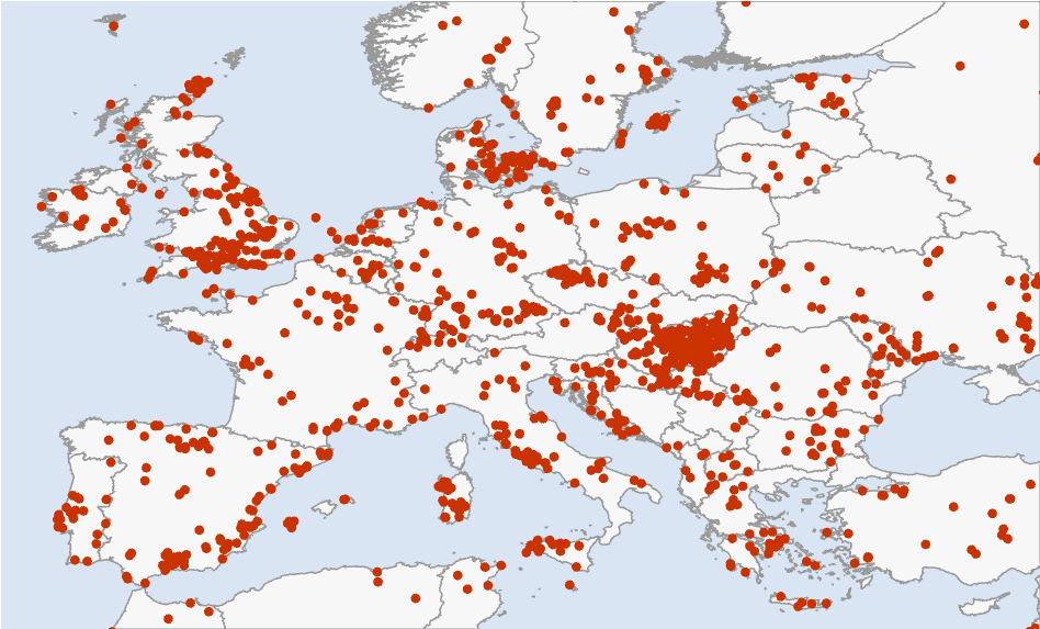
Where the 10119 usable ancient individuals come from. Density is wildly uneven in space and time — the Mediterranean is rich, the Baltic sparse, and almost nothing is younger than 2,500 years — and that unevenness is exactly why the model must carry its uncertainty around explicitly.
2. What is lactase persistence?
2. What is lactase persistence?
Lactose, the sugar in milk, cannot be absorbed directly: it must first be split into glucose and galactose by the enzyme lactase, produced in the lining of the small intestine and encoded by the LCT gene. In the ancestral mammalian program, lactase production is switched off after weaning — an adult wolf, cow, or (ancestrally) human who drinks milk gets bloating, cramps, and worse, because undigested lactose ferments in the colon. The European persistence variant is not a change to lactase itself: it is a single C→T substitution 13,910 bases upstream, inside an intron of the neighbouring gene MCM6, that acts as an enhancer and simply keeps the LCT switch turned on into adulthood. On the reported strand of the association database this is the G→A change at rs4988235 — one letter, one glass of milk, and (as we will see) several percent of extra surviving children per generation at its peak.
External asset. The gene schematic was generated outside Wolfram Language with OpenAI's gpt-image-2 model; the prompts and the one-off Python driver are checked into docs/images/figures-generated/ of the project repository. It is a static illustration; there is no WL code to run for this figure.
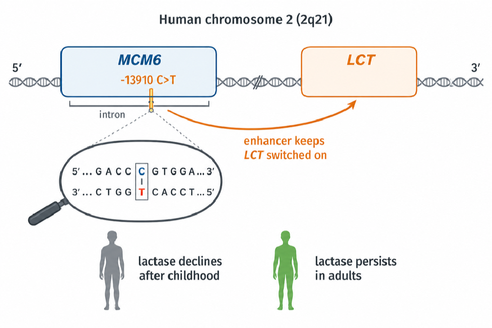
A crucial subtlety for what follows: the variant is effectively dominant — one copy is enough to digest milk — and it rides on a long shared haplotype, which is how it was first detected from modern data alone. But modern data compress history: they can say the allele rose fast, not when. Ancient DNA turns the same question into direct observation.
External asset. The ancient-DNA workflow illustration was generated outside Wolfram Language with OpenAI's gpt-image-2 model; the prompts and the one-off Python driver are checked into docs/images/figures-generated/ of the project repository. It is a static illustration; there is no WL code to run for this figure.
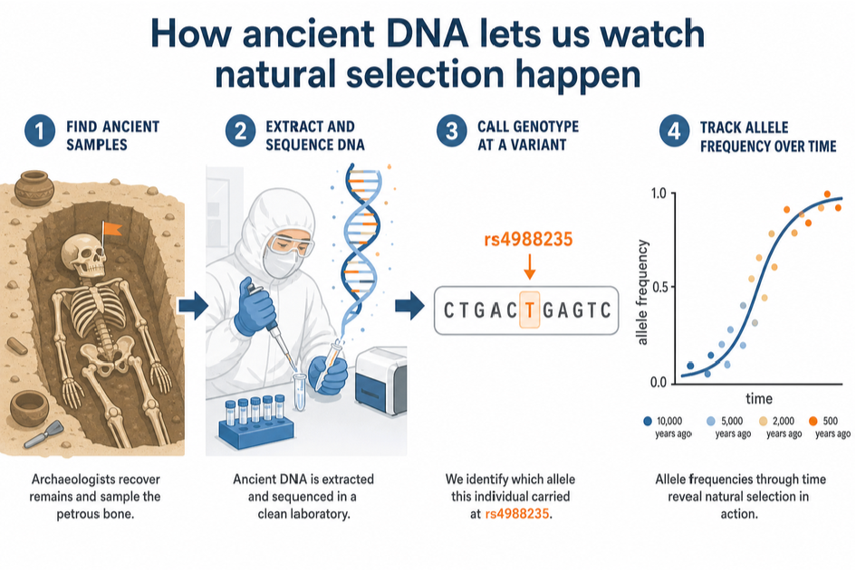
3. The regional story: four binomial logistic fits
3. The regional story: four binomial logistic fits
Before any spatial machinery, the honest first step is to reproduce the standard non-spatial description: for each region, a logistic trajectory logit p(t) = α + β (10000 − t)/1000 fitted by maximizing the exact binomial log-likelihood over every called allele — no time-binning enters the fit; the bins you see in the figure are display only, each carrying a 95% Wilson score interval and sized by its allele count. Standard errors come from the numerical Hessian at the optimum, and the fitter flags any solution that lands on a parameter bound. That flag is not decoration: an early version of this project silently reported a boundary solution for the British Isles, and the only symptom was a suspiciously round α. Fits you cannot audit are fits you cannot trust.
Out[]=
region | samples | alleles | derived | α | β per kyr | ≈s per gen |
British Isles | 803 | 1050. | 410. | -8.72 ± 0.63 | 1.07 ± 0.08 | 0.030 |
Rhine-Danube | 3370 | 4269. | 705. | -10.64 ± 0.64 | 1.09 ± 0.07 | 0.031 |
Mediterranean | 1437 | 1768. | 94. | -7.87 ± 0.78 | 0.67 ± 0.10 | 0.019 |
Baltic | 414 | 768. | 247. | -10.14 ± 1.03 | 1.16 ± 0.12 | 0.033 |
With a 28-year generation time, a slope β on the logit scale translates to an approximate per-generation (genic, codominant) selection coefficient s ≈ 28β/1000. The four regions land between 0.019 and 0.033 — the familiar few-percent picture, strongest in the north-west. Burger et al.'s 0.06 is estimated over the last three millennia only, while these slopes average over eight, so it should and does sit at or above the top of this range: time-averaging dilutes a late, strong pulse.
In[]:=
regionalOutputs=ExportRegionalFitOutputs[Directory[],samples,fits];Import[regionalOutputs["RegionalFigure"]]
Out[]=
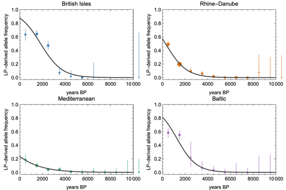
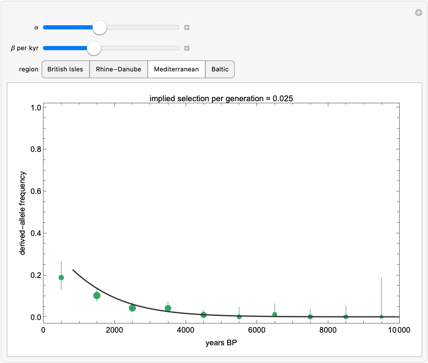
Observed binned frequencies (Wilson 95% intervals, point area ∝ allele count) with the fitted logistic curves. Note the Mediterranean's leisurely rise against the British and Baltic sprints — and note also how far right of the last data point every extrapolation to the present runs. Everything after ~2,000 BP is extrapolation, and the spatial model below inherits that caveat.
Rather than take my word for how sensitive these curves are, drag them yourself. The Manipulate below overlays an adjustable logistic on each region's binned data — the label converts your β into an implied selection coefficient as you drag. It takes about ten seconds of play to internalise two things: how narrow the corridor of plausible β is for the data-rich Mediterranean, and how wide it is for the Baltic.
In[]:=
LogisticExplorer[samples]
Out[]=
Static snapshot — evaluate this cell in a downloaded copy of the notebook to explore it interactively. |
4. A spatial diffusion–selection model
4. A spatial diffusion–selection model
Regions are administrative conveniences; alleles do not respect them. The spatial model discretizes Europe (35–63°N, 12°W–35°E) into a 2° grid, keeps only cells whose centres are on land (191 of them — so Britain stays rook-connected to the continent across the Dover cells, while Ireland becomes an island in the model's adjacency too, a caveat worth knowing), and lets the local allele frequency evolve in 250-year steps from 10,000 BP:
p[i, t+dt] = p[i, t] + g ( (s0 + sDairy D[i, t] m[region i]) p (1 - p)
+ mig mean[ p[j, t] - p[i, t], j adjacent to i ] )
g = dt / 28 generations per step
+ mig mean[ p[j, t] - p[i, t], j adjacent to i ] )
g = dt / 28 generations per step
Selection has a baseline component s0 and a component sDairy switched on by a smoothly varying dairying-onset field D(i, t) — built by inverse-distance interpolation from six regional anchor dates (Mediterranean ~8200 BP through Baltic ~5600 BP) rather than four flat plateaus, so the covariate has genuine spatial texture. Per-region multipliers m let the north run hotter than the south, and the migration term exchanges frequency with adjacent land cells. Here is the model's actual geography — the land cells it evolves on, coloured by when dairying arrives in each:
The model's spatial skeleton: the 2° land cells (sea cells are removed by an elevation test, so diffusion respects coastlines — Britain stays connected across the Dover cells, Ireland is an island in the adjacency too), coloured by the smooth dairying-onset field. Red is early dairying (Mediterranean and the southeast, ~8,200 BP), blue is late (the Baltic, ~5,600 BP). This field is what the sDairy component of selection switches on, cell by cell, as the simulation runs.
The covariate's shape in time is worth ten seconds of interaction too:
One forward simulation of this model costs about 70 ms:
— and that number is the entire strategy. When a simulator is this cheap, you do not need to linearize, approximate, or hand-wave the likelihood: you can afford tens of thousands of honest forward runs and let simulation-based inference do the rest. The model deliberately keeps demography implicit; it is a reaction–diffusion caricature whose job is to let the data say how much spatial structure, movement, and dairying-modulation they can constrain — not to smuggle conclusions in through the architecture.
External asset. The Neolithic dairying scene was generated outside Wolfram Language with OpenAI's gpt-image-2 model; the prompts and the one-off Python driver are checked into docs/images/figures-generated/ of the project repository. It is a static illustration; there is no WL code to run for this figure.
5. Inference: sequential Monte Carlo ABC
5. Inference: sequential Monte Carlo ABC
Approximate Bayesian computation asks the only question a simulator can answer: which parameters produce synthetic data that look like the real data? "Look like" is made precise through summary statistics; here, two families. First, the called-allele-weighted regional time-binned frequencies (37 bins). Second — because a spatial model scored only on regional aggregates can never learn about migration — each sample is matched to its nearest grid cell and time step, and pooled north−south and west−east frequency contrasts over the last 4,000 years are computed identically for observed alleles and model expectations. The distance is a weighted root-mean-square over all of it.
Plain rejection ABC wastes almost every simulation once the tolerance gets interesting, so the fit uses sequential Monte Carlo: a population of 400 particles is filtered through 6 generations of shrinking tolerance (each generation's ϵ is the median of the previous population's distances), with Gaussian perturbation kernels and importance weights. One implementation lesson worth passing on: with a 11-dimensional box prior, perturbing in the raw coordinates throws ~98% of proposals out of the box (0.7 to the 11th ≈ 0.020). The sampler therefore works in logit-transformed coordinates, where a uniform prior becomes an exact product of standard logistic densities, every proposal is automatically valid, and the importance weights stay closed-form.
The tolerance falls from 0.155 (the prior median — i.e. no information) to 0.040 over roughly 23000 simulations. The final effective sample size, 36.2 of 800, deserves a sentence rather than a footnote: importance-weight degeneracy is the known cost of this weight formula whenever the posterior is much tighter than the prior, every interval in this post is a weighted quantile and correspondingly approximate, and the honest cure — dropping the summaries altogether for the exact per-sample likelihood — is what §12 does. Reporting ESS is what separates a posterior from a scatter plot.
Weighted SMC posterior (blue) against the flat prior (dashed orange) for every parameter. Prior overlays are the fastest honesty check in Bayesian workflow: one glance separates the dimensions the data actually moved (initial frequency, dairying-modulated selection, the northern multipliers) from the ones still wearing their priors (the initial spatial gradients).
6. What the posterior says
6. What the posterior says
The last column is the anti-self-deception device: the posterior 95% interval's width as a share of the prior's. A value near 1 means the data taught us nothing about that parameter and its row is a restatement of the prior; only rows well below 1 are findings. Reviewers of an earlier draft of this analysis demonstrated — correctly — that several “agreements with the literature” were prior tautologies of exactly this kind, which is why the column now appears in every parameter table.
Three readings, in decreasing order of confidence. First, the total effective selection in a northern dairying cell at the posterior median — s0 + sDairy × multiplier ≈ 0.032 per generation — sits squarely in the published few-percent range, with the northern multipliers pulled above one exactly where the logistic slopes were steepest. Second, the posterior does not cleanly separate dairying-modulated from baseline selection. This is not a failure of the sampler; it is the geometry of the problem. The dairying covariate saturates to one within a few centuries of onset, so for most of the simulated period sDairy acts almost exactly like uniform selection; only the early Neolithic carries contrast between the two. That the ancient genotypes accommodate both a mostly-uniform and a mostly-dairy-modulated reading is this little model's echo of Evershed et al.'s conclusion at Nature scale: milk exploitation is not required to explain the trajectory. Third, migration is only weakly identified — §9 quantifies exactly how weakly, instead of letting a prior masquerade as a discovery.
7. The posterior on the map — and its uncertainty
7. The posterior on the map — and its uncertainty
Every map below is a posterior functional: 100 equally-weighted posterior draws, each pushed through the forward model, summarized per cell, then interpolated for display by ordinary kriging (range 3.5°, nugget 0.02) and cut to the coastline. Kriging here is a display courtesy, not an inferential claim — the 2° cells remain the units that saw data. Colors are the TemperatureMap scale with a square-root stretch so the long rare-allele centuries stay legible.
Posterior mean (top) and 95% credible-interval width (bottom) at 3000 BP. The two maps are a pair on purpose: the second is the error bar of the first, rendered at equal visual rank. The interval is widest exactly where the sampling map of §1 is emptiest — the model has the good manners to be unsure where it has seen nothing.
And because a static pair understates how the story unfolds, step through it yourself — each frame is the posterior mean with the ancient samples of that moment:
8. Does it actually predict anything?
8. Does it actually predict anything?
A posterior that merely redescribes its training data is a compression algorithm, not a model. Three checks, in increasing order of severity.
Posterior predictive. Push posterior draws through the model, sample binomial allele counts at each bin's actual sample size, and ask how often the observed frequency lands inside the 95% band: 97% of the 37 bins. Bins with two called alleles correctly get bands covering nearly everything — wide honesty beats narrow fiction.
Held-out regions. Refit the entire SMC from scratch four times, each time deleting one region's samples, then predict the deleted region:
Held-out time — the killer test. Train only on samples at or older than the 3,000 BP bin edge (4459 of them) and predict the 12 most recent bins. The intervals still cover, but the posterior median under-predicts the final rise badly (RMSE 0.33). Far from being embarrassing, this is the pipeline independently rediscovering Burger et al.'s headline: the evidence for strong, late selection is concentrated in the last three millennia. Delete those millennia and the model, sensibly, refuses to believe in them.
9. Which conclusions survive the priors?
9. Which conclusions survive the priors?
Five complete refits: baseline; halved selection priors; doubled migration prior; and every dairying onset shifted 400 years earlier or later. The dairying-modulated selection component stays positive in all five (medians 0.006–0.018) — though §11 will temper how much of that is data rather than the non-negative prior. The migration posterior tracks whichever prior it is given (median 0.007 baseline → 0.013 under the widened prior): with 191 cells and regionally-pooled summaries, movement is weakly identified, and the honest statement is exactly that.
10. Where did the allele come from? Origin versus selection
10. Where did the allele come from? Origin versus selection
Everything so far answers "where did selection push hardest?" — which is a different question from "where did the allele come from?", and the two are easy to conflate when watching the animation. The classic origin estimate is Itan et al. (2009), whose demic coevolution simulations placed the start of the lactase-persistence/dairying story around 7,500 years ago in the zone between the central Balkans and central Europe — roughly the Linearbandkeramik world of modern Hungary, Slovakia, and Austria. What do the ancient genotypes in this dataset say about first appearances?
The oldest derived-allele calls within the modelled era (≤ 10,000 BP), from the AADR v66 release. Read this table with suspicion, not reverence: most rows are single sequencing reads, and G→A is the very transition that post-mortem damage produces, so an isolated early “carrier” is as likely chemistry as biology — which is why the model fits an explicit error rate rather than taking the table at face value. The cautionary tale is what happened to the previous version of this table: under the 2021-era data behind our first fit, the three oldest carriers formed a tidy southeastern arc (Bulgaria ~6,560 BP, Ukraine ~5,600 BP, Romania ~5,390 BP). Current data dissolve two of the three — the Ukrainian individual has been redated to ~3,985 BP and the Romanian heterozygote is now called GG from the diploid genotypes — leaving one depth-2 heterozygote from Bulgaria carrying what was once a whole origin narrative.
The hero animation cannot show any of this, by construction: its model starts at 10,000 BP with a near-uniform initial frequency, has no mutation event, and — with migration weakly identified — moves essentially by in-place logistic growth. Britain lights up first there because its late samples demand the fastest growth, not because the allele originated there. So let us stop hand-waving and put the origin into the model: replace the uniform start with a point source. Six new parameters: origin latitude, longitude and time (time prior 5,000–10,000 BP, wide enough that both Itan et al.'s 7,441 BP and the ~6,000 BP rise date of Irving-Pease et al. live inside it); the injection frequency; a genotype-error rate ϵ ∈ [0, 0.02], because G→A is exactly the transition that post-mortem deamination fakes, and a model without an error channel is forced to treat every damaged Palaeolithic read as a real carrier; and a dairying lead time. That last one is the scientific commitment, made explicit and fitted rather than hidden in the prior: the source may not precede the local dairying onset by more than the lead (prior 0–2,000 years; origins after local onset are unrestricted — the constraint is deliberately asymmetric), because the thing being located is the start of the selection-driven rise, not the first mutation event — the same gene–culture coupling Itan et al. build into their model. Without it, a drift-free simulator lets a vanishingly small injection idle for millennia in pre-dairying forager regions. Migration gets a wider prior than the main model (a travelling wave has to actually travel: m ∈ [0.02, 0.3] per generation, capped where the mixing map saturates), the integrator uses exact per-step logistic growth with exponential mixing, and diagonal adjacency lets the wave cross the Dover strait. The same SMC machinery then turns "where did it start?" into a posterior distribution:
The decisive columns are the last two: the same quantiles under the CONSTRAINED PRIOR (the prior after the land and dairying-lead support restrictions, sampled by scripts/sample_constrained_prior.wls with no genetic data at all), and the posterior-to-prior width ratio. A posterior statement only carries information where it differs from that baseline. Read ruthlessly: the origin date's posterior median sits within fifty years of its constrained-prior median — the “published-envelope date” is generated by the archaeological chronology in the constraint, not by the genetics. What the genetic data actually move: the longitude (prior median 14.8°E → posterior 2.3°E) and, modestly, total selection strength. Most other rows are their priors.
The reverse-diffusion result, in the spirit of Itan et al.'s famous origin map: weighted posterior density of the point source's location, land-masked. Read the spread, not the star. §11 shows that this posterior is broad and multimodal enough that its mode is not a stable quantity — move the kernel bandwidth or reshuffle the resampling seed and the starred cell jumps between southwestern France, northern Germany and Iberia, a range of some 1,500 km. The star marks the modal cell of one particular kernel estimate; it is not a location estimate, and §11 makes the case that this posterior has no defensible point summary of location at all.
A prior-free cross-check on the same question: every non-origin parameter is pinned at its posterior median, the point source is placed in each land cell in turn, and the map is coloured by how well the forward simulation then matches the ancient samples (warmer = better fit). Read it honestly, in both directions. The well-fitting region is broad: the ancient data constrain the origin's latitude band far more sharply than its longitude, and because the northwest of the map is sampled most densely, the conditional optimum leans that way. But what the scan rules out is just as informative — Iberia, the southern Balkans, and the far northeast fit distinctly worse — and the posterior concentration above sits comfortably inside the preferred band. Where the joint posterior differs from this scan — most visibly in pulling mass away from regions where dairying arrived late — the difference is the gene–culture coupling and the joint fitting of origin time and injection frequency, not the origin prior, which is uniform over the whole map.
And the forward story from that fitted origin — the travelling wave the hero animation could not show — as its own video (the star marks the posterior modal origin; the inset again tracks the 95% credible-interval width):
Read the origin posterior with the same discipline as everything else here. The location information comes from a handful of early single-heterozygote calls scattered over an unevenly sampled map, filtered through a coarse deterministic wave model — so the credible region is wide, and it should be. What the fit adds beyond the anecdotal table above is that all three ingredients are now estimated jointly: an origin location and time, a wave that must actually reach Britain and the Baltic in time for their observed rises, and selection on top. Whether the posterior mass sits over the Carpathian Basin, the lower Danube, or the Pontic steppe is exactly the kind of statement this machinery exists to make — and unlike a caption, it comes with its uncertainty attached.
11. Checked against the published record
11. Checked against the published record
A model that only agrees with itself is not worth posting, so this section tests the fit against estimates it never saw. The benchmark is Itan et al. (2009) — a demic coevolution simulation driven by archaeological settlement dates and modern allele frequencies, with no ancient genotypes at all. Our fit uses only ancient genotypes. The two are largely — not entirely — independent: our gene–culture coupling consults the same archaeological dairying chronology that drives their simulation, so the origin-date comparison shares an input, while the genetic data are disjoint. That still makes the comparison worth doing — and worth doing numerically, not by putting two pictures next to each other and inviting the eye to find agreement. Two maps that share a warm patch can still be quantitatively far apart, and here they are.
So the first step is to turn their figure back into numbers — in Wolfram. Their Fig 3 carries tick marks at known latitudes and longitudes, so the pixel grid can be georeferenced exactly (the parallels are horizontal; the meridians converge northward at 35.85 px/degree along the top frame and 42.15 along the bottom), and the filled contour bands run along a blue–cyan–green–yellow–red ramp that inverts analytically. ImportItanFig3Density in the package does all of this in about forty lines of image processing; an independent Python implementation (scripts/digitise_itan_fig3.py) agrees with it to a mean absolute difference of 0.002 on the unit ramp scale. Two caveats are stated rather than hidden. First, the paper publishes no numeric colour scale, so equal density spacing between contour bands is an assumption; mode locations are robust to any monotone recolouring, but the overlap statistics below are approximate. Second, the paper's text localises the origin only qualitatively (“between the central Balkans and central Europe”); the coordinate 48.5°N, 14°E quoted in this section is the mode of our own georeferenced digitisation, not a number from their text. With both posteriors as numbers on one grid, the comparison becomes arithmetic:
Highest-posterior-density contours for both analyses on common axes — derived numeric contours only, no part of the published image reproduced. Itan et al.'s 50% region (blue, solid) is a compact ellipse over Bavaria, Bohemia and the Carpathian Basin. Ours (red, solid) sprawls from the Atlantic coast of France to Ukraine in several disconnected lobes, and our 95% region covers essentially the whole domain. This is the comparison the side-by-side view flattered.
The honest verdict on location. If the two posteriors were describing the same belief, the mass we place inside their 50% and 95% regions would be about 0.50 and 0.95. It is nothing like that. The last row is the one that is easy to misread: their whole distribution sits inside our 95% region, but that is a statement about how vague we are, not how right. A posterior wide enough to contain every rival hypothesis has not corroborated any of them.
Figure 3 of: Itan Y, Powell A, Beaumont MA, Burger J, Thomas MG (2009), “The Origins of Lactase Persistence in Europe”, PLoS Computational Biology 5(8): e1000491, doi:10.1371/journal.pcbi.1000491. © 2009 Itan et al., distributed under the Creative Commons Attribution (CC BY) licence (creativecommons.org/licenses/by/4.0), which permits unrestricted reproduction provided the original author and source are credited. Reproduced here unmodified; separately, the figure was digitised into the numeric density field used above (a derived work under the same licence). It shows the posterior density of the origin of the lactase-persistence/dairying coevolution in their demic model, with the high-density region running from Bavaria/Bohemia toward the Carpathian Basin — the “Hungary result” of the popular retellings.
Parameter by parameter, with the constrained prior kept in view. The date: our median of 6650 BP [5121, 8845] overlaps Itan et al.'s 7,441 [6,256–8,683] — but so does the constrained prior (median 6,603 BP), so the overlap is supplied by the archaeological chronology, not the genotypes, and it should not be counted as an independent confirmation. Selection: the posterior total [0.023, 0.061] tightens the constrained prior's [0.007, 0.068] by excluding the weak tail — the genuine genetic content here — and sits inside Bersaglieri's wide 0.014–0.15, below Itan's dairyers-only [0.0518, 0.159], above Irving-Pease's genome-wide 0.0194; Burger's ≈0.06 is estimated assuming dominance, which this genic model does not implement, so that comparison is indicative only. Location is where honest trouble lives, and marginal medians hide it: a marginal median is a poor summary of a broad multimodal joint posterior, and quoting one here would manufacture agreement the joint distribution does not support.
One more check, at the other end of time: extrapolate the fitted uniform-start model to the present (0 BP, i.e. 1950) and compare with today's measured rs4988235-A frequencies from the 1000 Genomes Project at the four sampled populations that sit on our grid:
Present-day extrapolation versus 1000 Genomes phase-3 allele frequencies (Ensembl). Everything after ~2,000 BP is extrapolation far beyond the ancient data, and the wide intervals say so. The second table is the test that keeps everyone honest: it scores the model's medians against the laziest imaginable null — predicting 0.5 for every population. A spatial diffusion–selection machine that cannot clearly beat a constant has no present-day predictive content, whichever way the comparison lands in the build you are reading; the model is calibrated for the ancient window it was fitted to, and that is the only window it should be quoted for.
Taken together, measured against the constrained prior that is the only fair baseline: the origin date is not a genetic finding — its posterior tracks the constrained prior, whose archaeological chronology already generates the published date range on its own. Total selection strength is a modest genuine finding: the posterior excludes the weak tail the prior allows (width ratio ≈0.6), landing in the published few-percent territory, though comparisons across studies remain inexact (Burger et al.'s 0.06 assumes dominance, which this genic model does not implement; Itan et al.'s applies to dairyers only). Location is not identified; the one real update is westward — mass west of 5°E roughly doubles from its constrained-prior 27% to ≈58% (±8% Monte Carlo, ESS 36) — and that lean must be read alongside three unremoved westward biases: northwest sampling density, the grid's latitude-dependent geometry, and the absence of drift. The Carpathian box ends up genuinely undetermined: prior 3.4%, posterior bounded only below ≈8%. This analysis should not be cited as ancient-DNA evidence for OR against the Carpathian origin — and an analysis that can say precisely why it cannot answer the question is the more useful artifact.
Which assumptions decide the answer? If importing Itan et al.'s commitments one at a time drags the posterior east, the westward lean is an artefact of our assumptions; if nothing drags it east, the localization in their result must live in their data. Four complete refits (scripts/run_origin_bridge_experiments.wls), each changing exactly one thing against the baseline: trust the early calls (error rate forced to ≈0, so every damage-suspect early read counts as a real carrier); tight coupling (dairying lead capped at 200 years — the origin is the dairying front, the structural core of the demic model); slow mixing (migration capped where the travelling wave keeps memory of its source); and the last two together as the closest structural analogue of Itan et al.'s model that this framework can express:
The bridge table, read with its error bars on. Two hard caveats first. With effective sample sizes of 12–43, a reported Carpathian mass of 0 only bounds that mass below roughly 3/ESS (rule of three): about 8% at ESS 36 and 25% at ESS 12 — and since the constrained prior itself puts only 3.4% there, these fits have no power to exclude a Carpathian origin at all. And the KDE modes, quoted to half a degree, sit inside a disclosed instability of ~1,500 km; one variant's mode even lands on Mallorca, uninhabited at the modelled date — a reminder that the location surface is closer to noise than to signal. What the table does support: none of the three Itan-style assumptions this framework can emulate generates a central-European concentration on its own; every variant keeps most of its mass in the west, against a constrained-prior baseline of 27% west of 5°E. That is evidence that, within this model family, the emulated assumptions are not what produces Itan et al.'s localization — it is NOT evidence against a Carpathian origin, and their result additionally differs from ours in inputs we cannot emulate here (the modern allele frequency surface, drift, demic demography). Recovering a genuine localization from ancient DNA alone would need either far more pre-6000 BP genomes than biology left behind, or arrival-time statistics that read the spread geometry — the first item on the future-work list.
12. Letting every sample speak: the exact likelihood
12. Letting every sample speak: the exact likelihood
Everything above inferred parameters by ABC: simulate, compress the simulation into a few dozen regional time-bin frequencies, keep the parameter vectors whose summaries land within a shrinking tolerance of the observed ones. That machinery exists because most population-genetic simulators are stochastic and their likelihoods intractable. Ours is not. The wave model of §4 is deterministic: a parameter vector fixes the allele frequency p in every cell at every 250-year step, and each ancient individual is then a binomial draw from p at its own cell and date (through the genotype-error channel q = p(1−2e)+e). The likelihood is therefore exact, and it is a product over all 6034 in-era samples rather than over a handful of bins — no summary statistics, no tolerance schedule, no importance weights to degenerate. One evaluation costs one forward simulation:
That price makes plain MCMC affordable: an adaptive Metropolis sampler (Haario et al. 2001) in the same unbounded logit coordinates the SMC used, proposal covariance learned from the chain's own history, 30,000 iterations per chain, three chains from different seeds. The package call below reloads the stored main chain (data/processed/origin_mcmc_chain.csv) or runs it; the two extra chains come from scripts/run_origin_mcmc_chain.wls. Same origin model, same constrained prior as §10 — only the information extracted from the data changes:
Median and 95% interval under the constrained prior, the ABC posterior of §10, and the exact-likelihood posterior (main chain), with the ratio of the last two interval widths. The exact likelihood shrinks every interval by an order of magnitude. It also pins one parameter against a bound: 7% of the pooled draws put the British-Isles selection multiplier within 1% of its ceiling of 2.2 (OriginTimeBP, by contrast, sits at about 9066 BP, well inside its 10,000 BP bound). A parameter pinned to a bound is the model saying it cannot do something the data demand — here, make Britain rise fast enough — and it is the first warning sign, discussed below. And these are one chain's intervals; the convergence table below shows why that is not yet trustworthy.
The same map function as §10, fed the exact-likelihood chain. The diffuse Atlantic-leaning ABC cloud has collapsed onto the Alpine foreland. Do not read this as a discovery yet: the next two tables say why.
First, did the chains converge? Three chains, three seeds, split-R-hat (Gelman et al. 2013) per parameter and the per-chain effective sample size (Geyer's initial-positive-sequence estimator). R-hat near 1 means the chains agree; the modern threshold is 1.01, and by that standard — and by the target of a few hundred effective draws per chain — this run does not pass:
Convergence diagnostics across the three chains. Location agrees across chains (all three medians sit within a few degrees) but the selection multipliers do not: the worst split-R-hat is about 6.4 and the effective sample size bottoms out near 3 per chain, so the posterior is far from Gaussian and nowhere near enough samples. Read the map as a location that is robust across chains; do not read the single-chain 95% intervals in the table above as calibrated. A properly mixed sampler (differential-evolution or tempered) is on the list in §14.
Second, and more important: is the model any good? With an exact likelihood one can finally ask the question ABC cannot. The ladder below puts several models on the same 6034 samples: a constant frequency; five independent logistic curves in time, one per region, with no space at all; the spatial standing-variation model of §4 (allele present everywhere at 10,000 BP with a smooth gradient) at the best-fitting point its own exact-likelihood chains reached; the point-source model likewise; and the saturated model with one free frequency per occupied time×cell bin, the ceiling any model can reach. The last column is how many nats above the constant-frequency model each one buys — more is better, and the saturated value is the most any model on these data could reach:
The deviance ladder. Each spatial row is the best likelihood any of its chains reached, so it is a lower bound on that model's true maximum — the point-source chains span about 9 nats among themselves, a direct measure of how far from the optimum they are; the standing-variation gap below is wide enough to survive that slack. Read the middle rows against each other: the point-source model, with more likelihood parameters, still fits worse than five unrelated logistic curves, and the standing-variation model beats both. A single origin plus a diffusion wave is not merely unidentified by these data — it is a worse description of them than assuming the allele was already everywhere. (Columns count only parameters that enter the likelihood; DairyingLeadYears, which acts only through the support constraint, is excluded.)
Third, where does the point-source model lose? Splitting the log-likelihood difference between the point-source MAP and the regional logistic fit by region and millennium locates the damage:
Log-likelihood of the point-source model minus that of the regional logistic curves, in nats, by region and millennium BP. Blue: the spatial model does better; red: worse. The wave model wins by 68 nats in Rhine–Danube, where 3,000+ samples resolve genuine within-region structure that five curves cannot see, and loses 62 nats in the British Isles and 45 in the Baltic, almost all of it in the 1–2 kyr BP bins.
The British-Isles loss is instructive because the aggregate frequency there is nearly right (0.64 observed against 0.61 predicted for 1–2 kyr BP), so the model is not simply too low on average. The damage is within the region and it is concentrated: a handful of derived alleles land in cells the deterministic front has left near the error floor, and each one there costs several nats. A single continental wave with constant selection sharpens into a near-step front, so it cannot simultaneously be high in the south-east and high on the Atlantic and Baltic margins where early risers also appear; something local (stronger selection, a second source, or demography the model does not carry) is needed, and the British-Isles selection multiplier sitting on its ceiling of 2.2 is the model straining to say so. The parameters on their bounds tell the same story: Migration at 0.3 means the per-step mixing fraction α = 1 − exp(−8.9 m) is already 0.93 — the wave is as fast as the lattice allows — and the data still want it faster, i.e. they want the allele to appear nearly simultaneously across Europe. Pushed that way, a point-source model relocates its origin to the least-bad centroid of the sample cloud, which is what the Alpine-foreland star is. The standing-variation model says the same thing in its own coordinates: its chains put the allele at roughly 0.07% everywhere at 10,000 BP, slightly higher in the north, with slow mixing (Migration ≈ 0.033) — gradients are preserved rather than created.
The error-rate posterior tells the same story from the other end. At e ≈ 0.018 in the point-source chains the channel is no longer a damage rate; the model is using 1−e as a ceiling, because constant selection drives p to 1 while the data plateau near 0.6–0.7 (the standing-variation chains, which need no ceiling, settle at a plausible e ≈ 0.005). Lactase persistence is phenotypically dominant, so the natural fix is diploid selection with dominance h (fitnesses 1, 1+hs, 1+s): selection fades as the non-persistent homozygote becomes rare, and p plateaus on its own. The package now carries that recursion (DominanceGrowth), switched on by a "Dominance" parameter, and a 20,000-iteration chain with h free (scripts/run_origin_mcmc_dominance.wls) is the extra row in the ladder above: at a log-likelihood of -2879.9 it does not rescue the point-source model; this single, poorly-mixed chain lands at dominance h ≈ 0.68 (the biology expects near-dominance, h close to 1, and the plateau it buys does not close the gap) — and it moves the best-fit origin to 51.9°N, 6.4°E, about 750 km from the point-source estimate. A location that moves that far when the selection recursion changes is a property of the model, not of the allele.
One caution applies to the winner too. The standing-variation model wins the ladder, but its own two chains are no better mixed than the point-source ones (worst split-R-hat about 4.2, minimum effective size about 5 per chain), so the numbers quoted from it — the near-uniform starting frequency, the slow mixing — are the shape of its posterior, not tightly estimated values. What is robust is the ranking: the ladder gaps are tens of nats, far larger than the few-nat slack the chains leave, so which model fits better is not in question even though neither model's parameters are pinned down.
What survives. The exact likelihood does not overturn §10 and §11 — it sharpens them into a statement ABC could not make. Timing and the size of selection are stable across ABC, exact likelihood and all three chains. Location is identified by the exact likelihood, but only within a model the same likelihood rejects in favour of standing variation; a location estimate from a rejected model is not an estimate of where the allele arose. That is the honest end point of this dataset for the origin question, and it is a more useful one than a wide credible region: the next model has to let selection start locally and at different times in different places, which is exactly the archaeology of dairying.
13. The animation, assembled
13. The animation, assembled
The hero animation at the top of the post is the whole pipeline in one artifact: 81 time-interpolated frames of the kriged posterior mean, the moving window of ancient samples, a progress bar, and — non-negotiably — the credible-interval inset, so that even a viewer who reads nothing else cannot mistake the smooth colours for certainty. Because every frame is raster-composited over a single cached base map, the full render takes under a minute:
14. What this is not
14. What this is not
This is a calibrated caricature, and the caveats are part of the result. The regional logistic layer reproduces the published four-region picture qualitatively, not parameter-for-parameter. The simulator is deterministic — no genetic drift — which flatters the posterior's tightness; demography (the steppe migrations!) is implicit; Ireland is unreachable in the adjacency; radiocarbon uncertainty enters the bins as point dates; the final ESS of 36.2 keeps every interval approximate; and everything after ~2,000 BP extrapolates beyond the data; and the exact-likelihood chains of §12, sharp as they are, have not converged on the selection multipliers. Next steps, in rough order of value: diploid selection with dominance (DominanceGrowth, already in the package) fitted with the exact likelihood; region-specific selection onset tied to the dairying map instead of a single origin; a Wright–Fisher stochastic core or a beta-binomial overdispersion term; calibrated-date uncertainty propagated per sample; sample-level ancestry-aware likelihoods.
15. Reproducibility
15. Reproducibility
Everything — data retrieval with checksums, processing with provenance, fits, SMC, validation, sensitivity, every figure, the hero animation, and this notebook itself — regenerates from the repository:
git clone https://github.com/mthiel74/ancient-dna-lactase-spatial-wolfram
wolframscript -file scripts/run_pipeline.wls --particles 400 --generations 5
wolframscript -file scripts/run_origin_mcmc.wls 30000 10000
wolframscript -file scripts/run_origin_mcmc_chain.wls 2718
wolframscript -file scripts/run_origin_mcmc_chain.wls 1618
wolframscript -file scripts/run_main_mcmc.wls 314159
wolframscript -file scripts/run_main_mcmc.wls 2718
wolframscript -file scripts/run_tests.wls
wolframscript -file community/build_notebook.wls
Random seeds: main SMC 20260831, origin SMC 19470, constrained-prior sampler 271828, exact-likelihood MCMC 314159 / 2718 / 1618 (origin model) and 314159 / 2718 (standing variation), resampling seeds derived deterministically from draw counts — every stochastic result in this notebook is reproducible bit-for-bit from these. The package src/LactasePersistenceSpatial.wl (~2,900 lines) carries the entire workflow behind the one-liners in this post; 30 VerificationTests cover the parsers, the simulator, the summary statistics, the SMC machinery and the exact likelihood. Repository: mthiel74/ancient-dna-lactase-spatial-wolfram.
16. References
16. References
Data. This project is built on the Allen Ancient DNA Resource (AADR). Per the AADR's own guidance, three citations are owed: the AADR paper, the specific Dataverse version used, and the original publication behind every individual sample — the last is carried in the Publication column of every processed row (307 distinct source studies across the 10119 individuals). Only a single-variant (rs4988235) extract is redistributed here; the full genotype files are not. See DATA_LICENCES.md for the complete provenance and terms.
Mallick, S., Micco, A., Mah, M., et al. (2024). The Allen Ancient DNA Resource (AADR): a curated compendium of ancient human genomes. Scientific Data 11, 182. nature.com/articles/s41597-024-03031-7
David Reich Lab (2024). The Allen Ancient DNA Resource, version v66.p1 [dataset]. Harvard Dataverse, doi:10.7910/DVN/FFIDCW. doi.org/10.7910/DVN/FFIDCW
Evershed, R. P., et al. (2022). Dairying, diseases and the evolution of lactase persistence in Europe. Nature 608, 336–345. nature.com/articles/s41586-022-05010-7
Burger, J., et al. (2020). Low prevalence of lactase persistence in Bronze Age Europe indicates ongoing strong selection over the last 3,000 years. Current Biology 30(21), 4307–4315. cell.com/current-biology
Bersaglieri, T., et al. (2004). Genetic signatures of strong recent positive selection at the lactase gene. American Journal of Human Genetics 74(6), 1111–1120.
Irving-Pease, E. K., et al. (2024). The selection landscape and genetic legacy of ancient Eurasians. Nature 625, 312–320. nature.com/articles/s41586-023-06705-1
Itan, Y., Powell, A., Beaumont, M. A., Burger, J., Thomas, M. G. (2009). The origins of lactase persistence in Europe. PLoS Computational Biology 5(8), e1000491 (CC-BY; Figure 3 reproduced in §11).
The 1000 Genomes Project Consortium (2015). A global reference for human genetic variation. Nature 526, 68–74. rs4988235 population frequencies via Ensembl.
GLAD LP Ancient Genotypes 2022 workbook (UCL), derived from the Allen Ancient DNA Resource v44.3.
Analysis, figures, and notebook generated with Wolfram Language 15.0.1 on September 2, 2026.
CITE THIS NOTEBOOK
CITE THIS NOTEBOOK
Watching evolution happen: lactase persistence in 8,000 years of ancient DNA
by Marco Thiel
Wolfram Community, STAFF PICKS, September 2, 2026
https://community.wolfram.com/groups/-/m/t/3791183
by Marco Thiel
Wolfram Community, STAFF PICKS, September 2, 2026
https://community.wolfram.com/groups/-/m/t/3791183