Mathematica
Introduction
Introduction
This notebook (and other notebooks) were used in the presentation "Random mandalas deconstruction with R, Python, and Mathematica" given at "Boston useR! Meetup" in February 2022. Here is a link to presentation's recording.
Here is presentation's abstract:
In this presentation we discuss the application of different dimension reduction algorithms over collections of random mandalas. We discuss and compare the derived image bases and show how those bases explain the underlying collection structure. The presented techniques and insights (1) are applicable to any collection of images, and (2) can be included in larger, more complicated machine learning workflows. The former is demonstrated with a handwritten digits recognition
application; the latter with the generation of random Bethlehem stars. The (parallel) walk-through of the core demonstration is in all three programming languages: Mathematica, Python, and R.
application; the latter with the generation of random Bethlehem stars. The (parallel) walk-through of the core demonstration is in all three programming languages: Mathematica, Python, and R.
Remark: This is a Mathematica notebook with Wolfram Language (WL) code. There are corresponding notebooks with Mathematica/WL and R/RStudio with Python, R, and WL codes.
Workflow
Workflow
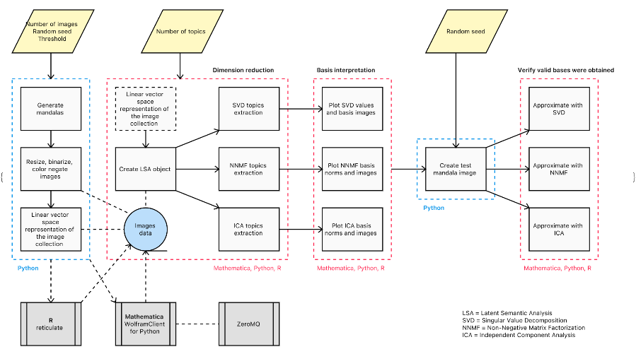
Here is a diagram that shows the overall process followed in all notebooks used in the presentation:
Out[]=
Get Python mandalas collection
Get Python mandalas collection
Setup
Setup
In[]:=
# "Standard" packages
import pandas
import numpy
import random
import io
import time
# Plotting packages
import matplotlib
import matplotlib.pyplot as plt
from mpl_toolkits.axes_grid1 import ImageGrid
# Image processing package(s)
from PIL import Image, ImageOps
# Random mandalas packages
from RandomMandala import random_mandala, figure_to_image
import pandas
import numpy
import random
import io
import time
# Plotting packages
import matplotlib
import matplotlib.pyplot as plt
from mpl_toolkits.axes_grid1 import ImageGrid
# Image processing package(s)
from PIL import Image, ImageOps
# Random mandalas packages
from RandomMandala import random_mandala, figure_to_image
In[]:=
pythonSession=First@Pick[ExternalSessions[],#["System"]=="Python"&/@ExternalSessions[]]
Out[]=
ExternalSessionObject

Mandala collection
Mandala collection
In[]:=
# A list to accumulate random mandala images
mandala_images = []
# Generation loop
random.seed(443)
tstart = time.time()
for i in range(512):
# Generate one random mandala figure
fig2 = random_mandala(n_rows=None,
n_columns=None,
radius=[8, 6, 3],
rotational_symmetry_order=6,
symmetric_seed=True,
connecting_function='bezier_fill',
face_color="0.",
alpha = 1.0)
fig2.tight_layout()
# Convert the figure into an image and add it to the list
mandala_images = mandala_images + [figure_to_image(fig2)]
# Close figure to save memoru
plt.close(fig2)
# Invert image colors
mandala_images1 = [ImageOps.invert(img) for img in mandala_images]
# Binarize images
mandala_images2 = [im.convert('1') for im in mandala_images1]
# Resize images
width, height = mandala_images2[0].size
print([width, height])
ratio = height / width
new_width = 200
mandala_images3 = [img.resize((new_width, round(new_width * ratio)), Image.ANTIALIAS) for img in mandala_images2]
print("Process time: " + str(time.time()-tstart))
mandala_images = []
# Generation loop
random.seed(443)
tstart = time.time()
for i in range(512):
# Generate one random mandala figure
fig2 = random_mandala(n_rows=None,
n_columns=None,
radius=[8, 6, 3],
rotational_symmetry_order=6,
symmetric_seed=True,
connecting_function='bezier_fill',
face_color="0.",
alpha = 1.0)
fig2.tight_layout()
# Convert the figure into an image and add it to the list
mandala_images = mandala_images + [figure_to_image(fig2)]
# Close figure to save memoru
plt.close(fig2)
# Invert image colors
mandala_images1 = [ImageOps.invert(img) for img in mandala_images]
# Binarize images
mandala_images2 = [im.convert('1') for im in mandala_images1]
# Resize images
width, height = mandala_images2[0].size
print([width, height])
ratio = height / width
new_width = 200
mandala_images3 = [img.resize((new_width, round(new_width * ratio)), Image.ANTIALIAS) for img in mandala_images2]
print("Process time: " + str(time.time()-tstart))
[640, 480]
Process time: 23.023240089416504
Get mandalas in Mathematica
Get mandalas in Mathematica
In[]:=
mandalas3=ExternalEvaluate[pythonSession,"mandala_images3"];Length[mandalas3]
Out[]=
512
Process random mandalas collection
Process random mandalas collection
Show one of the random mandalas:
In[]:=
mandalas3〚12〛
Out[]=

In[]:=
{imageSizeX,imageSizeY}=ImageDimensions[mandalas3〚12〛]
Out[]=
{200,150}
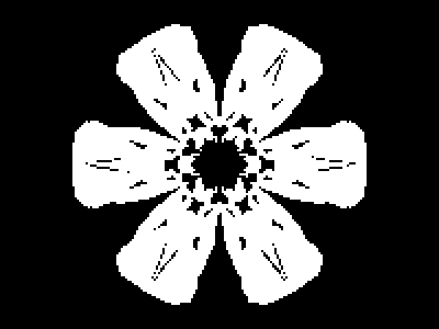
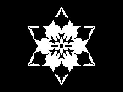
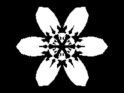
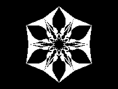
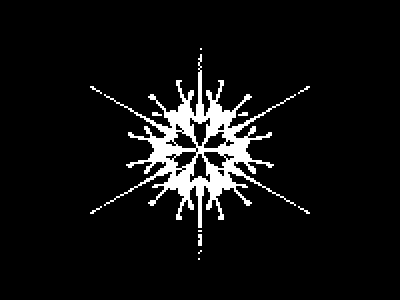
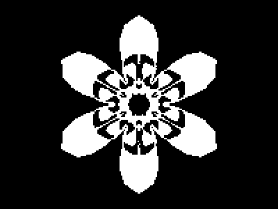
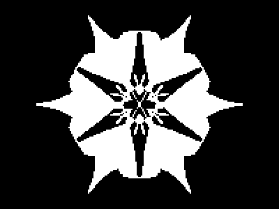
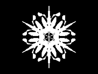
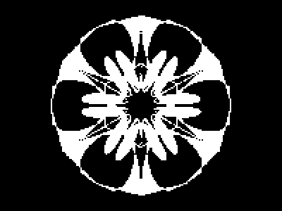
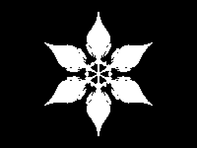
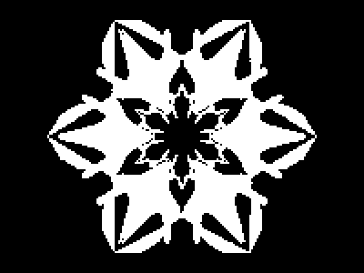
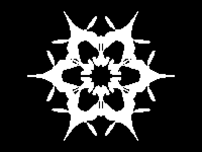
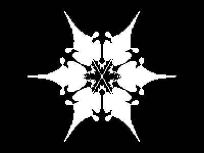
Show an array of inverted random mandalas:
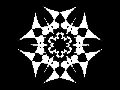
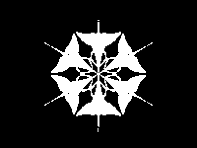
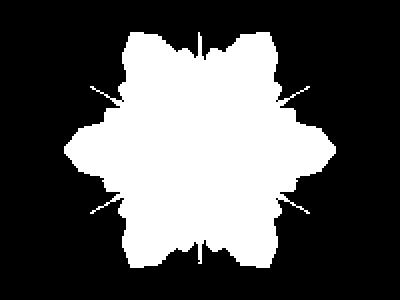
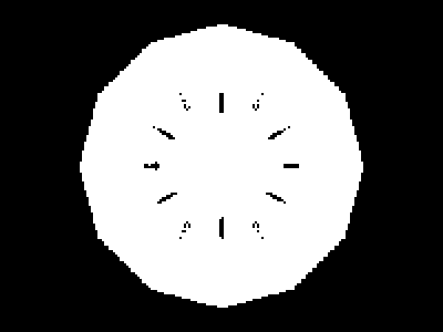
In[]:=
Multicolumn[RandomSample[mandalas3,36],6]
Out[]=







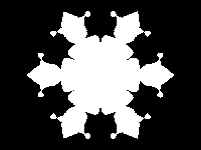
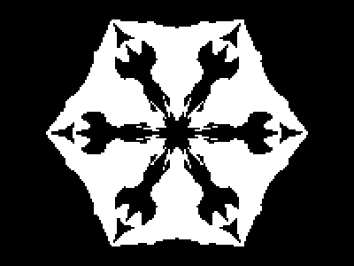



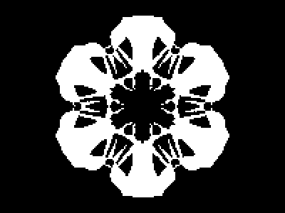
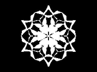

In[]:=
(*ResourceFunction["RandomMandala"]["SymmetricSeed"->RandomChoice[{True,False}],"RotationalSymmetryOrder"->3,ImageSize->Large,opts]*)
In[]:=
Tally[ImageDimensions/@mandalas3]
Out[]=
{{{200,150},512}}
Convert each image into array and flatten that array:
In[]:=
mandalaArrays=Flatten[ImageData[#]]&/@mandalas3;Dimensions[mandalaArrays]
Out[]=
{512,30000}
Make a matrix of flattened mandalas:
In[]:=
mandalaMat=SparseArray[N@mandalaArrays]
Out[]=
SparseArray

Make the corresponding SSparseMatrix object:
In[]:=
mandalaSMat=ToSSparseMatrix[mandalaMat,"RowNames"->Automatic,"ColumnNames"->Automatic]
Out[]=
SparseArray
LSAMon object creation
LSAMon object creation
Se the number of topics:
In[]:=
numberOfTopics=40;
Create the LSAMon object:
In[]:=
AbsoluteTiming[lsaObj=LSAMonUnit[]⟹LSAMonSetDocumentTermMatrix[mandalaSMat]⟹LSAMonApplyTermWeightFunctions["GlobalWeightFunction"->"None","LocalWeightFunction"->"None","NormalizerFunction"->"None"];]
Out[]=
{0.071211,Null}
SVD
SVD
Here we extract image topics using Singular Value Decomposition (SVD):
In[]:=
AbsoluteTiming[lsaSVDObj=lsaObj⟹LSAMonExtractTopics["NumberOfTopics"->numberOfTopics,Method->"SVD","MaxSteps"->16,"MinNumberOfDocumentsPerTerm"->0];]
NNMF
NNMF
Here we extract image topics using Non-Negative Matrix Factorization (NNFM):
ICA
ICA
Here we extract image topics using Independent Component Analysis (ICA):
Show topics interpretation
Show topics interpretation
SVD
SVD
Show the importance coefficients of the topics (if SVD was used the plot would show the singular values):
Show the interpretation of the extracted image topics:
NNMF
NNMF
Show the importance coefficients of the topics :
Show the interpretation of the extracted image topics:
ICA
ICA
Show the importance coefficients of the topics :
Show the interpretation of the extracted image topics:
Approximation
Approximation
Get a new, unseen random mandala:
Get the generated mandala image in Mathematica:
Get the corresponding vector:
SVD
SVD
Represent by topics :
NNMF
NNMF
ICA
ICA