Problems including a charged wall producing an electric field and charged conducting sphere are common in introductory Electromagnetism classes. This project provides a way to visualize the changes in position and angle as variables (such as mass, charge, and insulating string length). As I am taking AP Physics II, visualizations like this help me to better understand relationships between variables without access to hands-on labs.
Developing the Simulation
Developing the Simulation
First, we will create the graphical representation of a wall, ball, and angle. All units are standard SI except for the ball’s charge which is in microcoulombs.
Initializing constants:
In[]:=
ballCharge=100;presetLocation={2,3.3};L=3;wallField=500;m=0.01;
Creating a charged wall:
In[]:=
chargeColor=;Chargelines={Thickness@.045,chargeColor,Table[Line[{{0,i},{1,i}}],{i,.5,5.5,.5}]};Wall={Black,Rectangle[{-.2,0},{1+.2,6}]};

Visualizing the wall by itself:
In[]:=
Graphics[{Wall,Chargelines}]
Out[]=
Creating a charged ball:
In[]:=
ChargedBall[charge_,location_]:={Ball[location,.3],Text[Style[charge,White,15],location-{0,.01}]}
Initializing charge, location for ball and adding it into visualization:
In[]:=
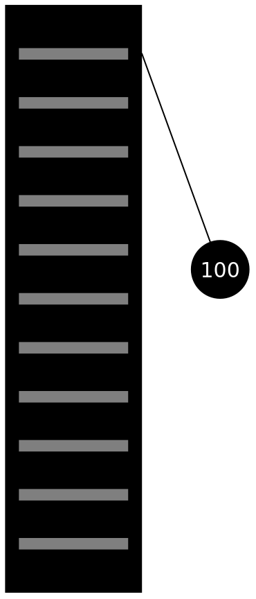
Graphics[{Wall,Chargelines,Line[{{1.2,5.5},presetLocation}],ChargedBall[ballCharge,presetLocation]}]
Out[]=
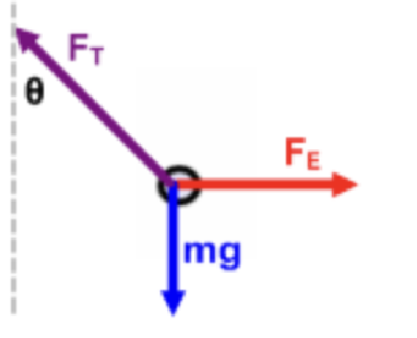
To find the angle between the insulating string and wall, I used . As shown in the graphic attached below, the horizontal electric force is equivalent to the horizontal component of tension and the weight is equivalent to the vertical component of tension, yielding the above formula. The weight of the ball is calculated by multiplying mass by g, 9.81. The electric force due to the wall is calculated by multiplying the electric field of the wall by the charge of the ball.
ArcTan[weightoftheball/electricforceexertedontheball]
Free-body diagram illustrating electric force and field (Progressive Science Initiative [PSI], n.d.):
Calculating angle between insulating string and wall:
In[]:=
theta[m_,E_,b_]:=ArcTan[(m*9.81),(E*b*10^-6)]rad=theta[m,wallField,ballCharge]
Out[]=
0.471365
It is also important for us to convert the value we get in radians to degrees for it to be more easily understandable in the graphical representation.
Converting radians to degrees:
In[]:=
deg=UnitConvert[Quantity[rad,"Radians"],"AngularDegrees"]
Out[]=
Creating angle representation on graphics:
In[]:=
ChargeAngle[radian_,degree_]:={Circle[{1.2,5.5},.5,{3Pi/2,3Pi/2+radian}],Text[Style[StringJoin["θ=",ToString[Round[degree,3]]],White,Background->Black,15],{1.2,5.5}-.05]}
So far, we have working representations for all parts of the simulation but have not included calculations for the x and y coordinates of the ball as it reaches equilibrium. Lets see what it looks like with relatively arbitrary constants.
Putting it all together:
In[]:=
ChargedWall2[ballCharge_,wallField_,location_,radian_,degree_]:={Wall,Chargelines,Text[Style[StringJoin["E=",ToString@wallField],White,24],{0.35,3.25}],Line[{{1.2,5.5},location}],ChargedBall[ballCharge,location],ChargeAngle[radian,degree]};Graphics[ChargedWall2[ballCharge,wallField,presetLocation,rad,deg]]
Out[]=
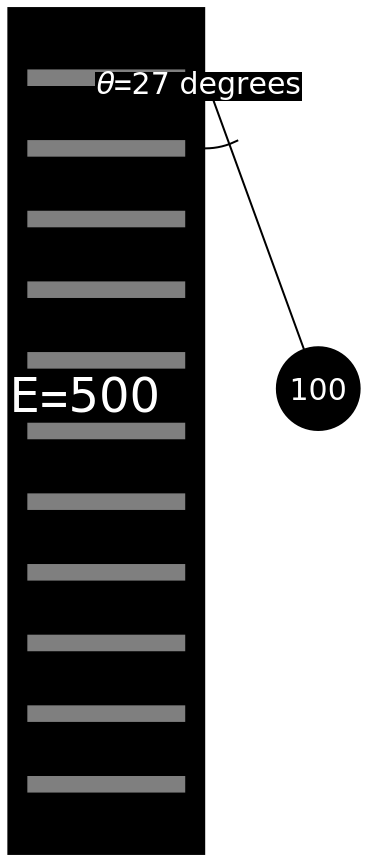
While this is somewhat close, it is obviously not completely accurate. The ball is in a slightly different position than what the angle would suggest. To calculate the balls horizontal position, we will add L*Sin(θ) and add that to the horizontal width of the wall. For vertical position, we will take the initial height and subtract it by L*Cos(θ).
Creating overall function which correctly calculates ball’s position:
In[]:=
WallSim[ballCharge_,wallField_,mass_,L_]:=Module[{x,y,location,radian,degree},radian=theta[mass,wallField,ballCharge];x=L*Sin[radian];y=L*Cos[radian];location={1.2+x,5.5-y};degree=UnitConvert[Quantity[radian,"Radians"],"AngularDegrees"];Graphics[ChargedWall2[ballCharge,wallField,location,radian,degree]]]WallSim[ballCharge,wallField,m,L]
Out[]=
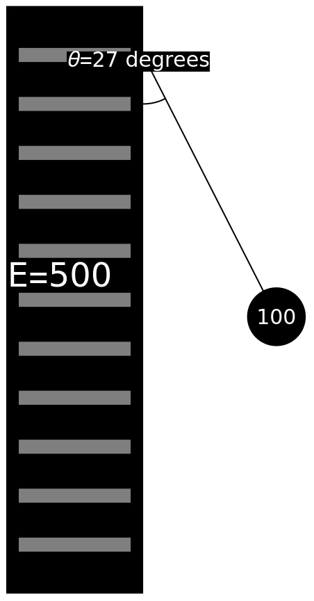
Animating how the ball gradually moves away from the wall:
Citations:
Citations:
Progressive Science Initiative (PSI®). (n.d.). Electric force & field: Free body diagram. AP Physics course materials. © All Rights Reserved.
Conclusion
Conclusion
Hopefully this helps to play around with various relationships in systems such as these. In the future, I hope to make a simulation to model how a ball reacts when the string is cut and it is allowed to accelerate away from the wall. Thank you for reading!
CITE THIS NOTEBOOK
CITE THIS NOTEBOOK
Simulating charged ball-wall system equilibrium
by Nikhil Mani
Wolfram Community, STAFF PICKS, October 25, 2024
https://community.wolfram.com/groups/-/m/t/3307740
by Nikhil Mani
Wolfram Community, STAFF PICKS, October 25, 2024
https://community.wolfram.com/groups/-/m/t/3307740