A nuclear reactor is typically a very highly contained vessel with stacks of nuclear fuel stacked within. A detector can be lowered through the axis of container and radiation at multiple points could be recorded. Data required for this would be synthetically generated using Monte-Carlo simulations based on a basic geometry, including a fuel pin, helium surrounding, Zircaloy cladding and water. The photons interactions have been studied and its lifetime is tracked from generation to termination.
Geometry
Geometry
Basic geometry considered for the simulations is as following. A single fuel pin consisting of Uranium dioxide,surrounded by helium jacket and a zircaloy cladding. The geometry shown below is the cross section of the fuel pin. In the other image the fuel pin and detector are shown. Not shown is the water region in between the fuel pin and the detector.

Random Generators
Random Generators
In Monte Carlo simulations randomness is very important. In this section all the necessary random generations are carried out from random generation of photon, its initial random direction, energy, etc. using RandomReal commands.
Random Position
Random Position
Shown is the random generation of 1000 photons inside the fuelpin.
InitialXYZ[f_]:=RandomPoint[f];data1=Table[InitialXYZ[fuel],{i,1,1000}];ListPointPlot3D[data1]
Out[]=

Random Direction
Random Direction
After the photons are generated they can travel in any random direction.The plot shows 1000 different ways in which
InitialdirectionGen:=(μz=RandomReal[{-1,1}];ϕ=RandomReal[{0,2*Pi}];Flatten[{μx=Sqrt[1-]*Cos[ϕ],μy=Sqrt[1-]*Sin[ϕ],μz}])data=Table[InitialdirectionGen,{i,1,1000}];ListPointPlot3D[data,AxesLabel{x,y,z}]
2
μz
2
μz
Out[]=

Data and Cross Section calculations
Data and Cross Section calculations
For the simulations cross section data is needed to calculate the probability of various interactions inside different regions for varying photon energies.
Number Density and Cross Section Data
Number Density and Cross Section Data
Number Density
Number Density
Atomic Density of Fuelpin, Helium, Zircaloy, Water.
ND["fuel"]=2.38*;ND["He"]=2.68*;ND["Zircaloy"]=1.5*;ND["water"]=3*;ND["Detector"]=2.5*;
22
10
22
10
22
10
22
10
22
10
Data for the cross section for all the materials and their respective interactions is obtained from the NIST XCOM website given in the reference. For some compounds the data is in /g units which need to be converted to /atomsbymultiplying by 10 and dividing by the atomic mass.
2
cm
2
cm
Uranium
Uranium
Cross Section function
Cross Section function
Sorting Cross Sections according to interactions and energy. Interactions included are Compton scattering, Photoelectric effect, Pair Production.
CrossSection[Z_String,r_]:=(Which[Z"fuel",csd=uranium,Z"He",csd=helium,Z"Zircaloy",csd=zr,Z"water",csd=wtr,Z=="Detector",csd=dtr];energy=csd[[1]];ne=Nearest[energy];scat=csd[[2]];photo=csd[[3]];pp=csd[[4]];cs=Merge[{AssociationThread[energy,scat],AssociationThread[energy,photo],AssociationThread[energy,pp]},Identity];First[Lookup[cs,ne[r]]])
Defined Functions
Defined Functions
Random length
Random length
Which region does the photon lie in?
Which region does the photon lie in?
Before each interaction the region where the photon is in is needed for finding the cross section.
WhichRegion[pos_]:=Which[RegionMember[fuel,pos],"fuel",RegionMember[He,pos],"He",RegionMember[Zircaloy,pos],"Zircaloy",RegionMember[Water,pos],"water",RegionMember[Outside,pos],"outside",RegionMember[Detector,pos],"Detector"]
Which interaction will happen?
Which interaction will happen?
Depending on the energy and the region of photon probability of each interaction is calculated.
In[]:=
WhichInteraction[Z_String,r_]:=(RandomChoice[{CrossSection[Z,r][[1]]/Total[CrossSection[Z,r]],CrossSection[Z,r][[2]]/Total[CrossSection[Z,r]],CrossSection[Z,r][[3]]/Total[CrossSection[Z,r]]}{"SC","PH","PP"}])
Direction after Scattering
Direction after Scattering
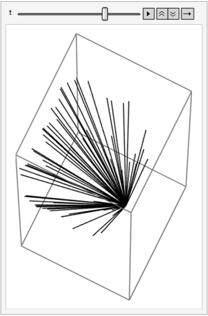
Direction Cosines after scattering of photon
INPUT : { direction cosines, theta, phi }
OUTPUT : direction cosines
INPUT : { direction cosines, theta, phi }
OUTPUT : direction cosines
Scattereddir[a_,θ_,ϕ_]:=Block{x,y,z},z=(a[[3]]*Cos[θ])+(Sqrt[1-]*Cos[ϕ]);x=((a[[1]]*(Cos[θ]-a[[3]]*z))-(a[[2]]*Sqrt[1-]*Sin[ϕ]))(1-);y=((a[[2]]*(Cos[θ]-a[[3]]*z))+(a[[1]]*Sqrt[1-]*Sin[ϕ]))(1-);{x,y,z};g=InitialXYZ[fuel];h=InitialdirectionGen;
2
a[[3]]
2
a[[3]]
2
a[[3]]
2
a[[3]]
2
a[[3]]
The GIF shows the different possible ways in which the photon can scatter after going through a Compton scattering event.
Running the simulation
Running the simulation
Taking together all the data and functions defined above the photons are tracked starting from birth till death one at a time.
Shown below is part of the code which is used for the simulation. During the photons run we would have to check if the photon crosses a boundary when travelling the random length. And if it is then we will have to take that point as initial and start the calculation again.This would be computationally expensive. Hence, here we have applied the Woodcock method in which the whole geometry is considered homogeneous with the cross section of the region which has the maximum value. To compensate for this bias at each point the interaction probability is divided by the maximum cross section.
Shown below is part of the code which is used for the simulation. During the photons run we would have to check if the photon crosses a boundary when travelling the random length. And if it is then we will have to take that point as initial and start the calculation again.This would be computationally expensive. Hence, here we have applied the Woodcock method in which the whole geometry is considered homogeneous with the cross section of the region which has the maximum value. To compensate for this bias at each point the interaction probability is divided by the maximum cross section.
ParallelTable[
pos = InitialXYZ[fuel];
dir = InitialdirectionGen;
ene = Energy;
sl = RandomLength[WhichRegion[pos], ene];
pos = Newxyz[pos, dir, sl];
(While[WhichRegion[pos] != "outside",
While[
RandomReal[{0, 1}, WorkingPrecision -> 10] > (Total[CrossSection[WhichRegion[pos], ene]]/Total[CrossSection["fuel", ene]]),
pos = Newxyz[pos, dir, RandomLength[WhichRegion[pos], ene]]
(*Print[pos]*)
];
Plots
Plots
Plot of the photons escaping the boundary
Plot of energy and the type of interaction which happens
Spread in energy as seen by NaI detector
Concluding remarks
Concluding remarks
The photon interactions including Compton Scattering, Photoelectric effect and Pair Production have been studied. Using this notebook, information about the photons specifically, the position and energy of the photons travelling from within the fuel cells can be recorded. Further, by modifying the geometry a leak can be simulated. For future work, we can train a classifier to identify a leak by looking at the data and also predict the approximate position of the leak.
Keywords
Keywords
◼
Monte Carlo
◼
Random Walk
◼
Reactor Physics
◼
Photon tracking
◼
Radiation
Acknowledgment
Acknowledgment
I would like to thank my mentor Varun Madhavan for all his guidance and support during this project. He has helped me develop practice of writing clean and efficient code. I would also like to thank Rahul Sharma, for answering my queries, although sometimes very silly ones.
References
References
◼
https://physics.nist.gov/PhysRefData/Xcom/html/xcom1.html for Cross section data.
◼
I. Lux, L. Koblinger, Monte Carlo Particle Methods: Neutron and Photon Calculations, CRC Press, Inc.,Florida, 1991.
◼
L.W.G. Morgan and D. Kotlyar. Weighted-delta-tracking for Monte Carlo particle transport. Annals of Nuclear Energy,85:1184–1188, 2015