Abstract: We construct a new entanglement witness out of connected two-particle reduced density matrix (C2RDM), that can probe whether a state is n-partite entangled. The new entanglement witness we construct can be measured through a combination of resonant inelastic X-ray scattering (RIXS) [1] and angle-resolved photoemission spectra (ARPES). In this project, we will explore the upper boundary of the entanglement witness for n-fermion state, deriving those upper boundary enables the functionality of the witness to tell whether N fermion states (N is large) is n-partite entangled or not.
Introduction
Introduction
Finding the measurable entanglement figure of merit is a crucial step towards detection and discovery of highly-entangled quantum materials, such as quantum spin liquids and unconventional high-Tc superconductors. The definition of entanglement entropy serves well to quantify the entanglement in computations, but it involves high-order or multi-point correlations that in the order of the system size, and it’s thus intractable in real experiments. With an upcoming new X-ray scattering spectra technique that we’ll soon post on arXiv [2], the measurable quantum correlations through spectra are extended from two-point correlations up to four-point correlations. In order to extract entanglement information from four-point correlations, we defined an entanglement witness based on connected four-point correlations (or connected two-particle reduced density matrix, referred as C2RDM in some literature). In this post, we will explore graphical ways to represent the entanglement witness for n-fermion state, that will assist the derivation of the upper boundary of the entanglement witness and also the understanding of general n-fermion state, which is mathematically much more complicated than n-qubit states.
Definition of Entanglement Witness
Definition of Entanglement Witness
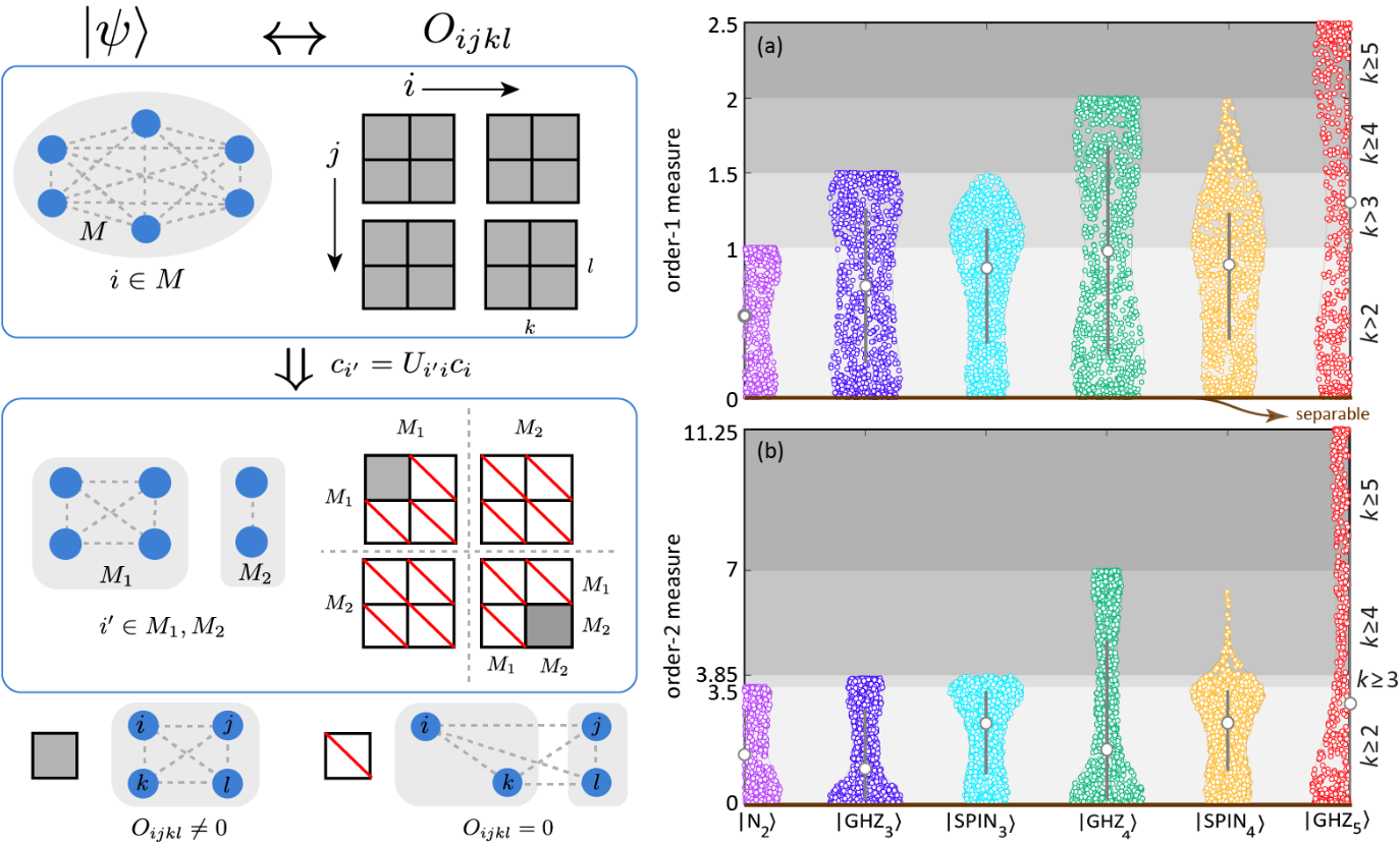
Experimentally, we will be able to measure the major components of the following correlation functions (we do not measure them in normal ordering in real X-ray experiments, but here we will assume normal ordering for simplicity, and it’s easy to make the transformation):In order to exclude the classical contribution from the four-point correlations, we take the connected part, and define rank-4 tensor as -+.The new entanglement witness is defined as the irreducible basic invariant of the tensor:Def: It has the following property that:Theorem: Given a pure state that can be decomposed as in any single-particle-orbital basis, where each ,,⋯,⋯ is the summation of products of creation operators that indicate a n-fermion states, then the irreducible basic invariant is a linear combination of the invariants of its separable subsystemsIn addition, a state whose largest block contain n fermions is called n-partite entangled, and it’s said to have multipartite entanglement to the depth n.An illustration of the above concept can be found in the left panel of this figure, and the right panel shows numerical simulation of for different classes of states, for more details of the concept and numerical simulations, please check my paper that is about to be posted, Therefore, if we can find the upper boundary of for n-fermion state, (n), we can use it as a multipartite entanglement witness, exceeding (n) indicate the system is at least (n+1)-partite entangled. It can be proved that (n)∼n and numerical results have shown that (n)∼n , and will tend to become a constant at large N, no matter how multipartite entangled the state is, so here we will focus on , In the following section, we will try to analysis this quantity for n-fermion state in different n, we will start from small like n=2,3,4, and explore the properties in a graphic form. The ultimate goal is to derive the upper boundary for each n, or even the upper boundary of for any , but we will start from some simple case and try to find clues to simplify the problem.
,,{i,j,k,l}∈N
†
c
i
†
c
j
c
k
c
l
†
c
i
c
j
O
ijkl
O
(ij),(kl)
†
c
i
†
c
j
c
k
c
l
†
c
i
c
l
†
c
j
c
k
†
c
i
c
k
†
c
j
c
l
F(O)Tr[],ν1,2,⋯
ν
O
ρ
ψ⋯|0
*
C
1
*
C
2
*
C
p
C
i
∑
{,,⋯,}
i
1
i
2
i
n
ω
i
1
i
2
i
n
†
c
i
1
†
c
i
2
†
c
i
n
F(O)
TrTrTr.
[]
ν
O
|ψ〉
ν
p
⊗
j1
O
*
C
j
p
∑
j1
ν
O
*
C
j
|ψ〉
*
C
j
Tr[O],Tr[]
2
O
Tr[]
ν
O
ν
F
N
n
ν
F
1
F
2
F
Tr[O]
N
Tr[]
2
O
Tr[]++-2|+2|-2|\[NewLine]+2|-2|
2
O
∑
ijkl
O
ijkl
2
|
∑
ijkl
†
c
i
†
c
j
c
k
c
l
2
|
†
c
i
c
l
†
c
j
c
k
2
|
†
c
i
c
k
†
c
j
c
l
2
|
†
c
i
†
c
j
c
k
c
l
†
c
i
c
l
†
c
j
c
k
†
c
i
†
c
j
c
k
c
l
†
c
i
c
k
†
c
j
c
l
†
c
i
c
l
†
c
j
c
k
†
c
i
c
k
†
c
j
c
l
∑
ijkl
†
c
i
†
c
j
c
k
c
l
2
|
†
c
i
c
l
†
c
j
c
k
2
|
†
c
i
c
l
†
c
j
c
k
†
c
i
c
k
†
c
j
c
l
n
Tr[]
ν
O
ν
Two-Fermion State n=2
Two-Fermion State n=2
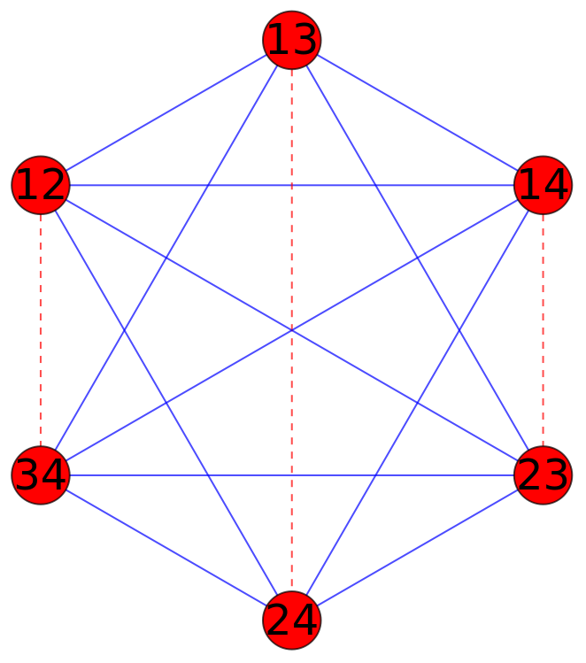
A general two-fermion statewhere is off diagonal matrix with element ,-,,the above transformation is valid for any antisymmetric matrix. Here, I will first consider the general case without applying the transformation, because the similar transformation does not work for fermion state with more than 2 particles. The correlations can be expressed aswhere represent all the permutation of index ia, and is the Levi-Civita tensor. What contributes to the is the pair of , and these crossing terms appear differently when and have distance 1, meaning they share one common element and each have one unique, or when and have distance 2 , meaning both elements are unique, note that here is an unordered set so the sequence does not matter. In order to represent it in a graphic form, I represent each unique as a dot in the graph, and an edge between and represent terms like , we label the dot as ij in the graph. There are two types of edges in the graph, one is when and have distance 2 and we represent them as red dashed lines, another is when and have distance 1 and we represent them as blue solid lines. The same definition of dots and edges in the graph also apply for later cases with different fermion number. We focus on a typical case when the system is half-filling (), so for n=2, N=4, there are 6 different dots representing
ω|0, ω↦Uωdiag[,⋯,,]
N
∑
i,j1
ω
ij
†
c
i
†
c
j
T
U
Z
1
Z
r
Z
0
Z
i
z
i
z
i
†
c
i
†
c
j
c
k
c
l
*
ω
[ij]
ω
[kl]
[ij]
ϵ
[kl]
ϵ
2
†
c
i
c
j
∑
a
*
ω
[ia]
ω
[ja]
[ia]
ϵ
[ja]
ϵ
∑
a
*
ω
ia
ω
ja
[ia]
ϵ
Tr[]
2
O
ω
ij
*
ω
′
i
′
j
{i,j}
{,}
′
i
′
j
{i,j}
{,}
′
i
′
j
{i,j}
{i,j}
{i,j}
{,}
′
i
′
j
*
ω
[ij]
ω
[]
′
i
′
j
[ij]
ϵ
[]
′
i
′
j
ϵ
{i,j}
{,}
′
i
′
j
{i,j}
{,}
′
i
′
j
n
N
1
2
2
C
4
{i,j}
In[]:=
(*Generatedistinctcombinationswithi<j*)dots=Select[Subsets[Range[4],{2}],#[[1]]<#[[2]]&];(*Defineafunctiontocheckiftwonodesshouldbeconnectedandhavedistance1*)distance1[{{i1_,j1_},{i2_,j2_}}]:=Length[Intersection[{i1,j1},{i2,j2}]]==1(*Generateallpossiblepairsofnodes*)distance1Edges=Select[Subsets[dots,{2}],distance1];distance2[{{i1_,j1_},{i2_,j2_}}]:=Length[Intersection[{i1,j1},{i2,j2}]]==0distance2Edges=Select[Subsets[dots,{2}],distance2];vertexMap=AssociationThread[dots->Range[Length[dots]]];(*Converteachlabelfrom{i,j,k}to"ijk"*)vertexLabels=StringJoin[ToString/@#]&/@Keys[vertexMap];(*Createanewmapforvertexlabeling*)vertexLabelMap=AssociationThread[Values[vertexMap]->vertexLabels];(*Convertedgestousethesenewidentifiers*)mappedDistance1Edges=distance1Edges/.vertexMap;mappedDistance2Edges=distance2Edges/.vertexMap;(*Defineedgestyles*)edgeStyles=Join[Thread[UndirectedEdge@@@mappedDistance1Edges->Blue],Thread[UndirectedEdge@@@mappedDistance2Edges->Directive[Red,Dashed]]];(*Nowcreatethegraph*)g=Graph[Values[vertexMap],Join[UndirectedEdge@@@mappedDistance1Edges,UndirectedEdge@@@mappedDistance2Edges],VertexLabels->Table[v->Placed[vertexLabelMap[v],Center],{v,Values[vertexMap]}],VertexLabelStyle->Large,GraphLayout->"CircularEmbedding",EdgeStyle->edgeStyles,VertexSize->Medium,VertexStyle->Red];Show[g]
Out[]=
Three-Fermion State n=3
Three-Fermion State n=3
we present the above graph in two different embeddings to show it more clearly. Next step we should consider whether such simplification allows the upper boundary to appears in the selected subset of basis.
Four-Fermion State n=4
Four-Fermion State n=4
Next step we should consider whether such simplification allows the upper boundary to appears in the selected subset of basis.
Concluding remarks
Concluding remarks
Keywords
Keywords
◼
Geometric information of Graph
◼
Entanglement Witness
◼
Quantum many-body physics
Acknowledgement
Acknowledgement
The author would like to thank Stephen Wolfram and Xerxes D. Arsiwalla for introducing this attractive project and help during the winter school. And thank my mentor Adiba Shaikh very much. Thanks all TAs and speakers for help and amazing talks. At last thanks all other staff members and students.
References
References
◼
L. J. P. Ament (2011), “Resonant inelastic x-ray scattering studies of elementary excitations”, Rev. Mod. Phys. 83, 705 , https://journals.aps.org/rmp/abstract/10.1103/RevModPhys.83.705
CITE THIS NOTEBOOK
CITE THIS NOTEBOOK
Multipartite Entanglement Witness with Four-Point Fermion Correlations
by Tongtong Liu
Wolfram Community, STAFF PICKS, January 11, 2024
https://community.wolfram.com/groups/-/m/t/3100855
by Tongtong Liu
Wolfram Community, STAFF PICKS, January 11, 2024
https://community.wolfram.com/groups/-/m/t/3100855