In this computational essay, we will explore how to apply Variational Quantum Linear Solver algorithm, proposed by Bravo-Prieto et al, in order to solve linear systems. We will compare results vs classical linear solver in Mathematica, and also symbolic and numeric quantum cases.
Paclet Installation
Paclet Installation
Wolfram quantum framework is a paclet. So first, let’s install it:
In[]:=
PacletInstall["https://wolfr.am/DevWQCF",ForceVersionInstall->True]
Out[]=
PacletObject

In[]:=
Get["Wolfram`QuantumFramework`"]
Load additional functions one needs for quantum variational linear solvers:
In[]:=
Needs["Wolfram`QuantumFramework`ExampleRepository`"]
Theory
Theory
The Variational Quantum Linear Solver (VQLS) is a a hybrid quantum-classical technique designed to address Quantum Linear Systems Problem (QLSP). It aims to find linear system solutions using quantum computing techniques. The corresponding quantum algorithm can be summarized as follows:
Given:
◼
A quantum state such that
|b〉
|b〉=U|0〉
◼
n
2
n
2
A
A=
L-1
∑
0
c
l
A
l
c
l
A
l
One wants to prepare:
◼
A quantum state such that and ->|b〉
|x〉
|ψ〉=A|x〉
|ψ〉
ψ
ψ
VQLS Approach
VQLS Approach
QLSP introductory example
QLSP introductory example
In this implementation we will consider the first qubit as our auxiliary qubit, since in the Wolfram QuantumFramework negative qubits and qubit 0 are used only for classical bits.
For this example we will consider a 2 qubits system plus an auxiliary qubit.
A=
X
2
H
3
|b〉=U|0〉=|0〉
H
2
H
3
where the operator’s index indicate the qubit it is applied on.
Given the ansatz:
|x〉=V(ω)|0〉=[()()]|0〉
R
y
ω
1
R
y
ω
2
H
2
H
3
We will proceed to build the circuit to minimize .
C
L
Circuit Implementation
Circuit Implementation
First we define the gates associated with the example:
The unitary matrix such that :
|b〉=|0〉
U
b
In[]:=
Ub=QuantumCircuitOperator[{"H"->{2},"H"->{3}},"Label"->""];
U
b
Because our goal is to conduct a Hadamard test, it’s necessary for the unitary operation to be controlled by the state of an auxiliary qubit:
A
In[]:=
ControlledAGate=QuantumCircuitOperator[{"CNOT"->{1,2},"CH"->{1,3}},"Label"->""];
A
2
Next, we implement the variational quantum circuit that generates a guess for :
|x〉
|x〉=V(ω)|0〉=[()()]|0〉
R
x
ω
1
R
x
ω
2
H
2
H
3
The first layer prepare an equal superposition of states and the second layer is the ansatz proposed before:
In[]:=
VariationalBlock=QuantumCircuitOperator[{"H"->{1,2},"RY"[ω1]->{1},"RY"[ω2]{2}},"Label"->"V(ω)","Parameters"->{ω1,ω2}];
In order to obtain we will implement a circuit that will deploy a Hadamard test:
μ
l,l',j
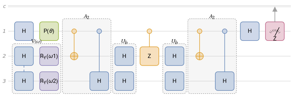
1. We first apply a Hadamard in the auxiliar qubit to prepare a state in superposition.2. We apply a Phase Shift to estimate the imaginary or real part of the μ: Re[μ] when θ 0 and Im[μ] when θ .3. Apply the Variational Circuit to generate a guess on .4. Apply the Controlled Gate corresponding to the component.5. Apply the adjoint , but in this case is the same as .6. Implement a controlled Z operator from the auxiliar qubit to the system qubit j. For the normalization calculation, we will use j = -1 to apply the identity.7. From this step, we will “undo” our operations, first by applying .8. Apply the Controlled gate‘s adjoint, which is the same as .9. Last Hadamard gate for the Hadamard testAt the end we apply a QuantumMeasureOperator to measure the expectation values.
-
π
2
|x〉
A
l
U
b
U
b
U
b
A
l
A
l
In[]:=
Clear[LocalHadamardCircuit];LocalHadamardCircuit[j_]:=QuantumCircuitOperator[{"Hadamard"->{1},"P"[θ],VariationalBlock->{2,3},ControlledAGate,Ub,If[!MatchQ[j,-1],"CZ"->{1,j},Nothing],Ub,ControlledAGate,"Hadamard"->{1},QuantumMeasurementOperator["Z"->{-1,1},{1}]},"Parameters"->{ω1,ω2,θ}]
You can test the multiple variations of the circuit for each controlled gate:
In[]:=
LocalHadamardCircuit[2]["Diagram",ImageSize->Large]
Out[]=
Optimized Circuit Implementation
Optimized Circuit Implementation
As you might notice, the past implementation might be slow if we want to obtain the expected value for each combination. Moreover, the local cost function that we will implement later to optimize will need to calculate the mean value multiple times.
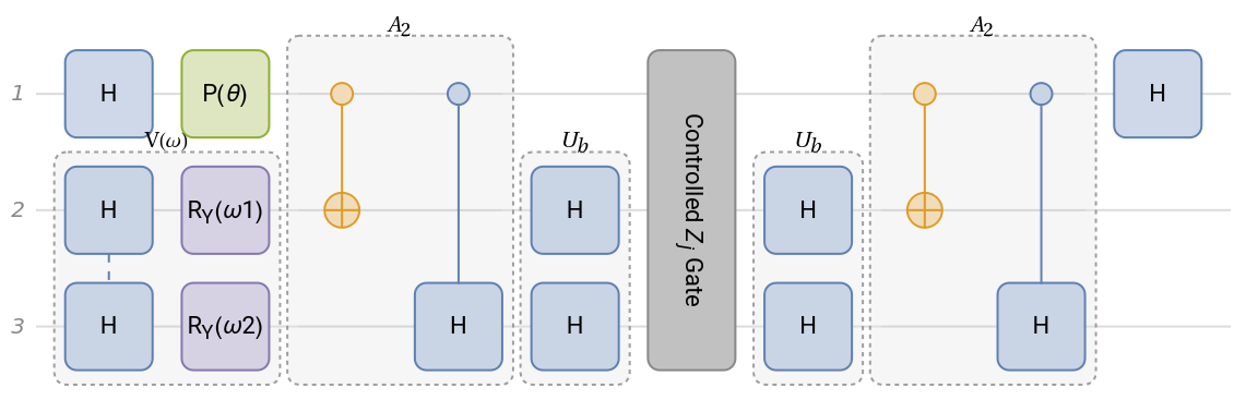
Instead we could try to use the useful KroneckerProduct to build the same circuit with all the variations.
We can re-implement gate, since it depends in which qubit it will be applied on:
CZ
In[]:=
ControlledGateZ=QuantumOperatorQuantumOperator["CZ"->{1,2}]*KroneckerDelta[j,2]+QuantumOperator["CZ"->{1,3}]*KroneckerDelta[j,3]+QuantumOperator["I"]*KroneckerDelta[j,-1],"Label"->"Controlled Gate";
Z
j
As you might notice, we just apply a KroneckerDelta to get rid of the qubits we won’t be using for each case, this is possible since we already know how many qubits we are working on.
As the previous subsection, we implement the Hadamard test:
In[]:=
ClearAll[LocalHadamardCircuit];LocalHadamardCircuit=QuantumCircuitOperator[{"Hadamard"->{1},"P"[θ],VariationalBlock->{2,3},ControlledAGate,Ub,ControlledGateZ,Ub,ControlledAGate,"Hadamard"->{1}},"Parameters"->{ω1,ω2,j,θ}];
Check out the newly implemented circuit diagram:
In[]:=
LocalHadamardCircuit["Diagram",ImageSize->Large]
Out[]=
Local Cost Function
Local Cost Function
We just obtained the Symbolic Mean value of our circuit, in order to replace the variables quickly we define the following function:
Now we will implement all the functions needed for the cost function defined in the Theory section:
Next, implement the normalization term:
Symbolic Cost Function Optimization
Symbolic Cost Function Optimization
Let’s calculate the symbolic equation for the cost function. It is not that huge of an expression, but surely not visually pleasant to show here:
Since we have the symbolic function, we can use NMinize:
Numerical Cost Function Optimization
Numerical Cost Function Optimization
We can use our previously defined LocalCost for numerical calculations using a numerical gradient descent:
Classical Linear System Solving
Classical Linear System Solving
Solve the system by operating over the correspondent matrices:
Finally, compute the probabilities:
Symbolic & Numeric Quantum Circuit Result
Symbolic & Numeric Quantum Circuit Result
Test the Variational circuit with the optimized parameters results:
The symbolic optimization resultant probabilities:
The numerical optimization resultant probabilities:
We can calculate how different one distribution is from another using a Kolmogorov Smirnov Test:
In this case, the number is considered big enough to indicate that the results are from the reference distribution.
Let’s plot the probabilities for a visual comparison:
QLSP implemented in Rigetti Quantum Computer
QLSP implemented in Rigetti Quantum Computer
This QLSP was already tested by Bravo-Prieto using Rigetti’s quantum chip 16Q Aspen-4.
For this example we will consider a 3 qubits system plus an auxiliar qubit.
where the operator’s index indicate the qubit it is applied on.
Given the ansatz:
Circuit Implementation
Circuit Implementation
As the previous QLSP, we define the gates associated with the example:
Local Cost Function
Local Cost Function
Now let’s calculate the symbolic mean value:
Finally we use the ket and bra obtained to calculate the expected value:
Now we will implement all the functions needed for the cost function defined in the Theory section:
Now we will implement the normalization term. In this case l and lp values correspond to our system qubits:
Symbolic Cost Function Optimization
Symbolic Cost Function Optimization
Let’s calculate the symbolic equation for the cost function. It is not that huge of an expression, but surely not visually pleasant to show here:
Since we have the symbolic function, we can use NMinimize:
Numerical Cost Function Optimization
Numerical Cost Function Optimization
We can use our previously defined LocalCost for numerical calculations using a numerical gradient descent:
Classical Linear System Solving
Classical Linear System Solving
Solve the system by operating over the corresponding matrices:
Finally, compute the probabilities:
Symbolic & Numeric Quantum Circuit Result
Symbolic & Numeric Quantum Circuit Result
Test the Variational circuit with the optimized parameters results:
The symbolic optimization resultant probabilities:
The numerical optimization resultant probabilities:
We can calculate how different one distribution is from another using the Kullback–Leibler divergence:
Since the results are small, it is an indicator that the distributions are similar.
We can also employ a Kolmogorov Smirnov Test:
In this case, the number is considered big enough to indicate that the results are from the reference distribution.
Let’s plot the probabilities for a visual comparison:
QLSP randomly generated
QLSP randomly generated
and we are given the state:
Given the ansatz
Circuit Implementation
Circuit Implementation
Following the same steps, we define the gates associated with the example:
Ansatz variational circuit:
As the previous example, we implement the Hadamard test:
Local Cost Function
Local Cost Function
Calculate the symbolic mean value of our function:
Now we will implement the functions to calculate the local cost for this circuit:
In this LocalHadamardMeanValues version, we call LocalHadamardStateVectors[{l, lp, j}] for the state vector already computed to save time per each execution of LocalCost:
Implement the normalization term:
Cost Function Optimization
Cost Function Optimization
We will calculate the gradient descent for our cost function:
Classical Linear System Solving
Classical Linear System Solving
Solve the system by operating over the correspondent matrices:
Finally, compute the probabilities:
Symbolic & Numeric Quantum Circuit Result
Symbolic & Numeric Quantum Circuit Result
We can build the Variational circuit from the example and test it with the optimized parameters result:
Test the Variational circuit with the optimized parameters results:
The optimization resultant probabilities:
We can calculate how different one distribution is from another using the Kullback–Leibler divergence:
Since the results are small, it is an indicator that the distributions are similar.
We can also employ a Kolmogorov Smirnov Test:
In this case, the number is considered big enough to indicate that the results are from the reference distribution.
Let’s plot the probabilities for a visual comparison:
References
References
◼
Bravo-Prieto, C., LaRose, R., Cerezo, M., Subasi, Y., Cincio, L., & Coles, P. J. (2019). Variational Quantum Linear Solver. arXiv. https://doi.org/10.48550/ARXIV.1909.05820
◼
Mari, A. Variational Quantum Linear Solver. PennyLane Demos. https://pennylane.ai/qml/demos/tutorial_vqls/
CITE THIS NOTEBOOK
CITE THIS NOTEBOOK
Variational quantum linear solver
by Sebastian Rodriguez
Wolfram Community, STAFF PICKS, May 22, 2024
https://community.wolfram.com/groups/-/m/t/3180154
by Sebastian Rodriguez
Wolfram Community, STAFF PICKS, May 22, 2024
https://community.wolfram.com/groups/-/m/t/3180154