Bode, Nyquist, and Nichols Diagrams of Second-Order Systems
Authors: Housam Binous and Ahmed Bellagi
Bode, Nyquist, and Nichols Diagrams of Second-Order Systems
Authors: Housam Binous and Ahmed Bellagi
Authors: Housam Binous and Ahmed Bellagi
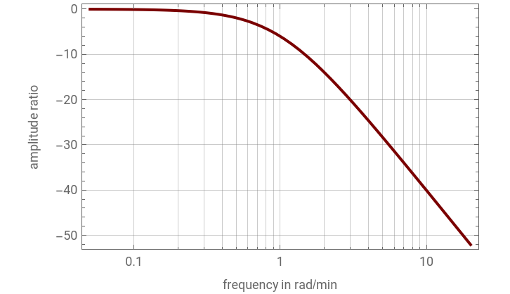
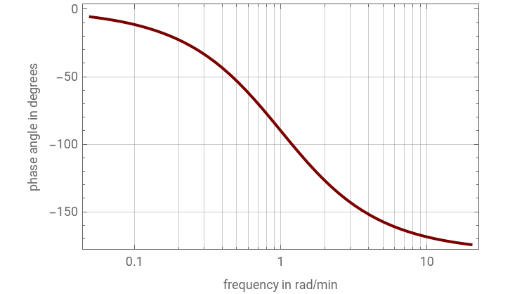
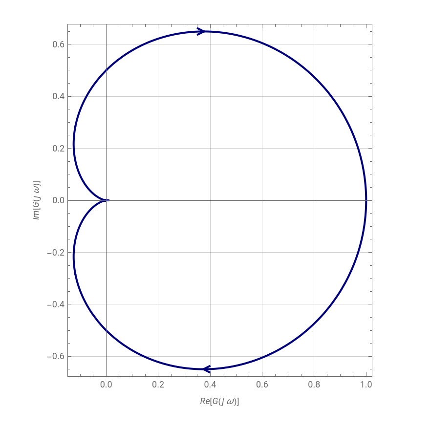
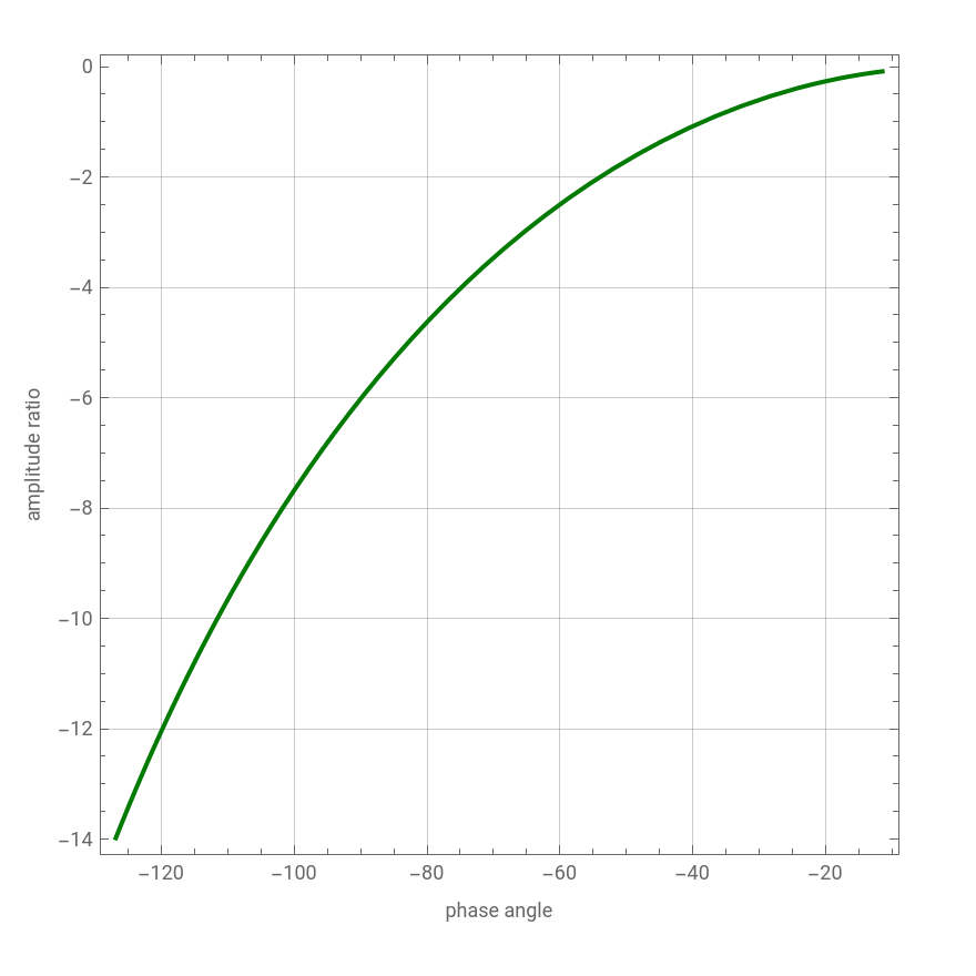
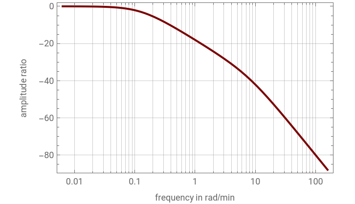
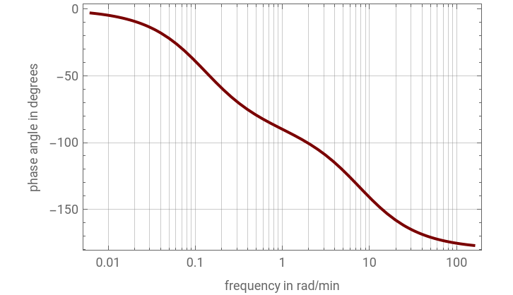
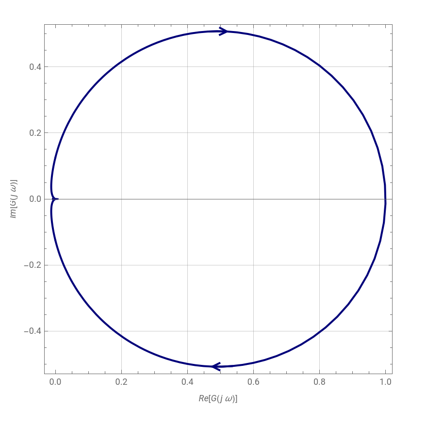
Consider a second-order system given by the transfer function:,where is the damping coefficient, is the response time, and is the process steady-state gain.We plots the Bode, Nyquist, and Nichols diagrams for user-set values of the parameters with =1, and .
G(s)=+2ζτs+1
K
p
2
τ
2
s
ζ
τ
K
p
ζ
K
p
τ=1
In[]:=
sys[k_,τ_,ζ_]:=TransferFunctionModel+2ζτs+1,s;
Kp
2
τ
2
s
In[]:=
(*gainKp*)Kp=1;(*responsetimeτ*)τ=1;
Different behaviors are observed for (underdamped or oscillating system), (critically damped system), and (overdamped system).
0≤ζ<1
ζ=1
ζ>1
In[]:=
(*criticallydampedsystem*)ζ=1;
In[]:=
BodePlot[sys[Kp,τ,ζ],PlotStyle{{Thick,RGBColor[0.48,0,0]},{Thick,RGBColor[0.48,0,0]}},GridLinesAutomatic,ImageSize1.1{{330,190},{330,190}},FrameLabel{{"frequency in rad/min","amplitude ratio"},{"frequency in rad/min","phase angle in degrees"}}]
Out[]=
In[]:=
NyquistPlot[sys[Kp,τ,ζ],FrameTrue,ImageSize1.1×400{1,1},GridLinesAutomatic,PlotStyle{Thick,RGBColor[0,0,0.48]},FrameLabel{Style["Re[G(j ω)]",Italic],Style["Im[G(j ω)]",Italic]},ImagePadding{{35,25},{55,25}}]
Out[]=
In[]:=
NicholsPlot[sys[Kp,τ,ζ],FrameTrue,ImageSize1.1×400{1,1},GridLinesAutomatic,PlotStyle{Thick,RGBColor[0,0.48,0]},FrameLabel{"phase angle","amplitude ratio"},ImagePadding{{35,25},{55,25}}]
Out[]=
In[]:=
(*overdampedsystem*)ζ=4;
In[]:=
BodePlot[sys[Kp,τ,ζ],PlotStyle{{Thick,RGBColor[0.48,0,0]},{Thick,RGBColor[0.48,0,0]}},GridLinesAutomatic,ImageSize1.1{{330,190},{330,190}},FrameLabel{{"frequency in rad/min","amplitude ratio"},{"frequency in rad/min","phase angle in degrees"}}]
Out[]=
In[]:=
NyquistPlot[sys[Kp,τ,ζ],FrameTrue,ImageSize1.1×400{1,1},GridLinesAutomatic,PlotStyle{Thick,RGBColor[0,0,0.48]},FrameLabel{Style["Re[G(j ω)]",Italic],Style["Im[G(j ω)]",Italic]},ImagePadding{{35,25},{55,25}}]
Out[]=
References :
[1] D. E. Seborg, T. F. Edgar, D. A. Mellichamp, and F. J. Doyle III, Process Dynamics and Control, 3rd ed., New York: John Wiley & Sons, 2010.
[1] D. E. Seborg, T. F. Edgar, D. A. Mellichamp, and F. J. Doyle III, Process Dynamics and Control, 3rd ed., New York: John Wiley & Sons, 2010.