In classical and quantum mechanics, symmetry plays a fundamental role in determining the behavior of physical systems. Symmetry in a system often leads to conserved quantities and simplifies the analysis of the system’s dynamics. However, when symmetry is broken, the system undergoes significant changes that can lead to new and fascinating phenomena. This analysis explores symmetry breaking in one, two, and three dimensional Hamiltonian oscillators along with quantum oscillators, focusing on the mathematical formulations and physical implications.
Introduction
Introduction
Symmetry is a fundamental concept in classical and quantum mechanics, deeply influencing the and properties of physical systems. In the context of Hamiltonian oscillators, symmetries lead to conserved quantities, which simplify the analysis and provide deep insights into the system’s dynamics. This study focuses on the breaking of various symmetries in one-dimensional (1D), two-dimensional (2D), three-dimensional (3D), and quantum Hamiltonian oscillators, such as time invariance and spatial uniformity, and explores the resultant physical implications.
This analysis will incorporate rotational and other symmetries, examining their role and the effects of their breaking on the dynamics of Hamiltonian and quantum oscillators. For 1D and 2D oscillators, we will investigate symmetry by analyzing angular momentum conservation and translational symmetry through the invariance under spatial translations. For 3D and quantum oscillators, we will extend these concepts to more complex scenarios, including spherical and quantum symmetry. The study will use canonical transformations and the Hamiltonian function to derive and understand the system’s behavior under symmetry breaking.
The primary aim of this research is to analyze the changes in the system’s equilibrium states and the emergence of new dynamical behaviors resulting from symmetry breaking. By conducting a detailed examination of the mathematical formulations and their physical interpretations, It is intended to provide a comprehensive understanding of the complex behaviors that arise in these systems.
Through this study, we will address the specific conditions under which symmetry breaking occurs, the nature of the new states that emerge, and the broader uses for similar systems.
The Harmonic Oscillator: 1D
The Harmonic Oscillator: 1D
Harmonic oscillators are widely seen throughout physics, representing systems like pendulums and masses on springs. They serve as fundamental models for a wide array of natural phenomena, where a restoring force proportional to the displacement from equilibrium acts. In classical mechanics, the motion of a harmonic oscillator is described by sinusoidal functions, managed by Hooke’s law for springs or the gravitational force for pendulums.
In a one-dimensional harmonic oscillator, spatial symmetry can be broken explicitly by introducing terms in the potential energy function that deviate from the standard quadratic form. For instance, adding cubic or higher-order polynomial terms to the potential function can break the original symmetry.
This leads to new dynamics and potentially complex behaviors in the system. Perturbations like these alter the potential landscape, causing the oscillator to behave in a non-linear manner. In the case of a harmonic oscillator, the equilibrium position is typically at with no initial velocity at 0. Introducing terms that break the symmetry modifies this equilibrium, leading to shifts in the position and altering the stability and behavior of the oscillator. This results in more complex, non-linear dynamics that differ significantly from the simple harmonic motion.
To further understand symmetry breaking in one-dimensional harmonic oscillators, we will establish the foundational dynamics of the one-dimensional harmonic oscillator.
This leads to new dynamics and potentially complex behaviors in the system. Perturbations like these alter the potential landscape, causing the oscillator to behave in a non-linear manner. In the case of a harmonic oscillator, the equilibrium position is typically at
x0
′
x
To further understand symmetry breaking in one-dimensional harmonic oscillators, we will establish the foundational dynamics of the one-dimensional harmonic oscillator.
First, we will define the Hamiltonian (a mathematical function involving coordinates and momenta (and possibly time)) for a one-dimensional harmonic oscillator and use the Poisson bracket (a mathematical operation that shows how the value of one function will change over time when the other function is considered as the Hamiltonian) to derive the equations of motion.
By understanding these basic equations, we can then explore how adding non-linear terms affects the system’s behavior, leading to symmetry breaking.
By understanding these basic equations, we can then explore how adding non-linear terms affects the system’s behavior, leading to symmetry breaking.
In[]:=
poissonBracket[A_,B_,x_,p_]:=D[A,x]* D[B,p]-D[A,p]* D[B,x];
In[]:=
hamiltonian=p^2/(2m)+k/mx^2;poissonBracket[x,hamiltonian,x,p];poissonBracket[p,hamiltonian,x,p]pdot=poissonBracket[p,hamiltonian,x,p];
Out[]=
-2x
To visualize the system’s fundamental dynamics, we will plot x and p on the x-p plane, which should form a circle for given values of E, k, and m. Additionally, we will plot x(t) and p(t) over time.
In[]:=
k=1;m=1;
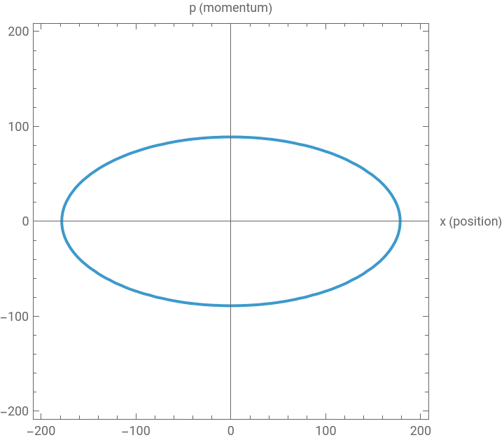
This plot shows the energy levels (contours) of the harmonic oscillator in the 𝑥-p plane, also known as phase space.
The equation (p^2/2m + 1/2 kx^2) represents an ellipse for different energy levels. The animation of this contour plot over different parameters (m, k) demonstrates how the phase space structure changes with varying energy levels and system parameters. The phase space trajectory (ellipse) represents the periodic motion of the oscillator, where each point on the ellipse corresponds to a state of the system at a given time (position and momentum).
The equation (p^2/2m + 1/2 kx^2) represents an ellipse for different energy levels. The animation of this contour plot over different parameters (m, k) demonstrates how the phase space structure changes with varying energy levels and system parameters. The phase space trajectory (ellipse) represents the periodic motion of the oscillator, where each point on the ellipse corresponds to a state of the system at a given time (position and momentum).
In[]:=
Animate[ContourPlot[p^2/(2m)+1/2kx^2==10000,{x,-200,200},{p,-200,200},Axes->True,AxesLabel->{"x (position)","p (momentum)"}],{m,0.001,1},{k,0.001,1},SaveDefinitions->True,AnimationRunning->False]
Out[]=
This plot shows the time evolution of the oscillator' s position x (t) and momentum p (t) . For a harmonic oscillator, x(t) and p(t) are sinusoidal functions of time, representing the oscillatory motion .
The animation shown below represents the periodic motion over time . The parametric plot (x (t), p (t)) forms a circle or ellipse, depending on initial conditions and system parameters . This visualization helps in understanding how the position and momentum of the oscillator evolve over time, emphasizing the periodic nature of simple harmonic motion .
In[]:=
Animate[ParametricPlot[{-10Sin[t],10Cos[t]},{t,0,tfinal},PlotRange->{-15,15}],{tfinal,0.1,10},SaveDefinitions->True,AnimationRunning->False]
Out[]=
We will then show the impact of adding a linear term to the potential energy of a one-dimensional harmonic oscillator, which provides insights into the new equilibrium points, potential energy landscape, and time evolution of the oscillator’s position, illustrating the effects of symmetry breaking on the system’s dynamics. The process for plotting and visualizing the impact is mainly a rinse-and repeat- like process, which consists of setting our parameters, defining the Hamiltonian, solving for the equations of motion, and plotting.
In[]:=
ω=1;λ=1;
In[]:=
HHH[x_,p_]:=p^2/(2*m)+(1/2)*m*ω^2*x^2
This plot visualizes the potential energy when symmetry is broken. As you can see, the potential energy increases significantly on the right-hand side, indicating broken symmetry.
Creates functions with broken symmetry, and finds their equilibrium, then plots it:
In[]:=
HsymmetryBroken[x_,p_]:=HHH[x,p]+λ*xV[x_]:=(1/2)*m*ω^2*x^2+λ*xxEquilibrium=Values[Solve[D[V[x],x]==0,x]][[1]];Show[Plot[V[x],{x,-5,5},PlotLabel->"Potential Energy with Equilibrium Points",AxesLabel->{"x","V(x)"},PlotRange->All],ListPlot[{#,V[#]}&/@xEquilibrium,PlotStyle->{Red,PointSize[0.02]}]]
Out[]=
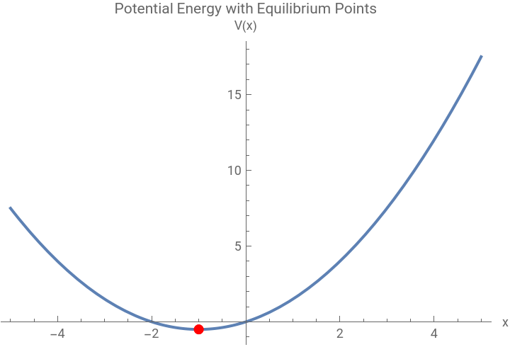
By adding an equilibrium point, we can view where the equilibrium is on the plot, showing where the symmetry actually changes, which further shows broken symmetry on a clearer level.
The Harmonic Oscillator: Symmetry in 1D
The Harmonic Oscillator: Symmetry in 1D
Time translational symmetry tests if the Hamiltonian remains unchanged under a time translation. This principle is fundamental in understanding energy conservation and the invariance of physical laws over time.
To test for time translational symmetry, we start by defining the Hamiltonian H of the system:
In[]:=
H=p[t]^2/(2m)+mω^2x[t]^2/2;
Next, we apply a time shift Δt to the position (𝑥[𝑡]) and momentum (𝑝[𝑡]) variables in the Hamiltonian . This results in a transformed Hamiltonian Ht :
Ht=H/.{x[t]->x[t+Δt],p[t]->p[t+Δt]};Simplify[H-Ht]
Out[]=
1
2
2
p[t]
2
p[t+Δt]
2
mω
2
x[t]
2
x[t+Δt]
If the Hamiltonian is invariant under this time shift, 𝐻 should equal Ht. Thus, the difference H − Ht should simplify to zero . We use the Simplify function to check this.
If it does, this confirms that the Hamiltonian is symmetric under time translation, indicating that the total energy of the system is conserved over time . By examining time translational symmetry in the harmonic oscillator, we gain insights into fundamental principles such as energy conservation and the invariance of physical laws over time .
Breaking Symmetry in 1D
Breaking Symmetry in 1D
In a perfectly symmetric 1 D harmonic oscillator, the Hamiltonian is quadratic in x and p . Introducing additional terms, such as cubic or other non - linear terms, breaks this symmetry . The cubic term and the complex term disrupt the harmonic potential, creating asymmetry that alters the oscillator’ s motion . Poisson brackets are used to derive the equations of motion from the Hamiltonian . They provide a way to compute the time evolution of the system’ s variables . The derived equations of motion [t](x,H)and[t](p,H)describe how the position and momentum evolve over time . Symbolic solutions provide exact expressions for and as functions of time, given the initial conditions . Numerical solutions are useful when the symbolic solutions are too complex or not easily obtainable, providing approximate solutions over a specified time range .
ax
3
[t]
sin(e(x[t)])
′
x
′
p
x[t]
p[t]
x[t]
p[t]
In[]:=
poissonBracket[A_,B_,x_,p_]:=D[A,x]*D[B,p]-D[A,p]*D[B,x];
In[]:=
cubicHamiltonian=(p[t]^2/(2m))+(kx[t]^2/(2m))+ax[t]^3;
In[]:=
pdot=poissonBracket[p[t],cubicHamiltonian,x[t],p[t]];xdot=poissonBracket[x[t],cubicHamiltonian,x[t],p[t]];
In[]:=
xdotpdot
Out[]=
p[t]
Out[]=
-x[t]-3a
2
x[t]
The Harmonic Oscillator: 2D
The Harmonic Oscillator: 2D
A two-dimensional harmonic oscillator extends the concept of oscillation into two perpendicular directions, typically represented as x and y coordinates. The symmetry in this system is typically rotational, meaning the system looks the same when rotated around the origin. To break this rotational symmetry, one can introduce terms in the Hamiltonian that couple the x and y coordinates or include non-linear terms in either coordinate. For example, a cubic term in one coordinate or cross terms like xy can disrupt the rotational symmetry, revealing greater depth within the system.
In exploring two-dimensional Hamiltonian oscillators, exploring energy surfaces within such systems.
Further exploring symmetry breaking, we will introduce some code that adds a cubic term in the Hamiltonian and animates the energy surface . This addition disrupts the rotational symmetry.
Pendulums
Pendulums
Like the harmonic oscillator, a pendulum exhibits periodic motion. For small angles, the motion of a pendulum can be approximated as harmonic, where the restoring force is proportional to the displacement from the equilibrium position .
The Hamiltonian of the pendulum system (considering small oscillations) is similar to that of the harmonic oscillator . Both systems have kinetic and potential energy terms that govern their dynamics . The solutions provided by the DSolve function for the harmonic oscillator are similar to the solutions for a pendulum’ s motion .
The parametric plots generated by the Animate function for the harmonic oscillator can be conceptually compared to the phase space plots of a pendulum . These plots help in understanding the periodic nature of the motion and the effects of varying parameters, in this case, tfinal and k.
The Harmonic Oscillator: 2D Symmetry
The Harmonic Oscillator: 2D Symmetry
In two-dimensional harmonic oscillators, rotational symmetry plays a crucial role in understanding the conservation laws associated with angular momentum and energy.
To explore rotational symmetry, we define the Hamiltonian H2D of the system :
Rotational symmetry in the 2D oscillator
Rotational symmetry in the 2D oscillator
Rotational symmetry refers to a property of an object or system that remains unchanged under rotations around a specified axis or point . In physics, rotational symmetry implies that the laws of physics managing the system are invariant under such rotations . Mathematically, rotational symmetry is often characterized by the preservation of physical quantities such as angular momentum or energy during rotational transformations .
To understand rotational symmetry, we start by defining the Hamiltonian and Poisson Brackets for the system :
Find the four differential equations using the Poisson bracket
Set parameters
Set Dsolve by using the 2 differential equations and using the two initial conditions
Compute the Hamiltonian to each value
To verify rotational symmetry, we use RotationTransform to rotate the coordinates and momenta by an angle θ :
Plot the difference between the rotated and original Hamiltonians to visualize the system’ s symmetry :
This plot visually demonstrates how the system’ s Hamiltonian changes under rotation, revealing any symmetry - breaking terms introduced by non-zero differences .
2D oscillator with diagonal term
2D oscillator with diagonal term
This plot represents the standard harmonic oscillator potential, symmetric in both x and y directions
The Hamiltonian is then defined for a 2D harmonic oscillator with a diagonal term.
Using the Poisson Brackets and DSolve, the equations of motion are derived and solved:
Whereas this animation visually demonstrates how the diagonal interaction modifies the system’s motion compared to the standard harmonic oscillator.
The difference between the two animations lies in the parametric equations used to describe the motion of the oscillator. The first animation uses terms with different coefficients and trigonometric functions, leading to distinct trajectories in the x-y plane. This variation showcases how changing the mathematical form of the coupling term affects the system’s dynamics, offering insights into the sensitivity of the oscillator’s behavior to alterations in its potential energy structure.
The Harmonic Oscillator: 3D Symmetry
The Harmonic Oscillator: 3D Symmetry
Motion in 3D: Solves and visualizes the motion of a 3D harmonic oscillator, demonstrating the periodic nature of the system in three dimensions.
Set initial Conditions:
Solve and Plot: (provides a numerical solution to the differential equations, essential for understanding how the oscillator’ s position evolves over time under specified initial conditions . )
Animate the trajectory:
The animated trajectory illustrates the periodic nature of the 3 D harmonic oscillator, exhibiting how initial conditions and parameters m and 𝜔 influence its trajectory in space .
The Quantum Harmonic Oscillator
The Quantum Harmonic Oscillator
Overview
Overview
In quantum mechanics, the harmonic oscillator is a foundational model used to describe a wide range of physical systems. The quantum harmonic oscillator is described by a Hamiltonian that includes kinetic and potential energy terms, where the potential energy is quadratic in the position.
Usage and Applications
Usage and Applications
Quantum harmonic oscillators find extensive applications across different fields of physics.
In quantum optics, they are crucial for describing the quantized modes of electromagnetic fields. These modes describe phenomena such as photon statistics, spontaneous emission, and the interaction of light with matter. In solid-state physics, quantum harmonic oscillators model the vibrations of atoms within a crystal lattice, known as phonons.
In quantum field theory, quantum harmonic oscillators are used to describe each mode of a field. Symmetry breaking in quantum field theory can lead to significant physical consequences, such as the Higgs mechanism in particle physics, where the spontaneous breaking of symmetry gives mass to fundamental particles.
The Quantum Harmonic Oscillator: Eigenfunctions and Eigenvalues
The Quantum Harmonic Oscillator: Eigenfunctions and Eigenvalues
What are Eigenfunctions and Eigenvalues?
Eigenvalues represent the quantized energy levels of the quantum harmonic oscillator, while Eigenfunctions represent the corresponding wavefunctions for these energy levels . The Eigenvalues provide the allowed energy levels of the system, which are discrete (quantized) rather than continuous . The Eigenfunctions describe the probability distributions of finding the particle at various positions .
Eigenvalues represent the quantized energy levels of the quantum harmonic oscillator, while Eigenfunctions represent the corresponding wavefunctions for these energy levels . The Eigenvalues provide the allowed energy levels of the system, which are discrete (quantized) rather than continuous . The Eigenfunctions describe the probability distributions of finding the particle at various positions .
Here, we calculate the Eigenvalues (vals) and Eigenfunctions (funs) of the Hamiltonian L over the interval 𝑥 ∈ [−5, 5] . Here, 5 specifies that we want to compute the first five Eigenvalues and corresponding Eigenfunctions .
We then plot and animate the Eigenfunctions, where each plot shows the probability distribution of finding the particle at different positions x .
And the Eigenvalues (where the Eigenfunctions (funs) are plotted for varying values of 𝑎 . This visualization helps to understand how the shape of the Eigenfunctions changes with respect to position 𝑥) we have obtained :
Symmetry In Quantum Harmonic Oscillators
Symmetry In Quantum Harmonic Oscillators
Symmetry in quantum oscillators, as in classical systems, simplifies the problem and leads to conserved quantities. For instance, in a spherically symmetric potential, the angular momentum is conserved.
Here is a simple example of symmetry in a quantum oscillator :
Plotting the Symmetric Harmonic Oscillator Wavefunctions :
The wavefunctions corresponding to the first five energy levels are plotted over the range −5 ≤ x ≤ 5. Each wavefunction is represented as a different curve, with the plot labeled to indicate that these are solutions for the symmetric quantum harmonic oscillator .
The wavefunctions corresponding to the first five energy levels are plotted over the range −5 ≤ x ≤ 5. Each wavefunction is represented as a different curve, with the plot labeled to indicate that these are solutions for the symmetric quantum harmonic oscillator .
These conserved quantities, such as angular momentum, not only stabilize the system but also provide quantum numbers that categorize energy levels and spatial orientations of wave functions. In practical terms, this means that in an atom or molecule with spherical symmetry, the electrons’ orbital angular momentum states remain stable and predictable.
Symmetry Breaking in Quantum Harmonic Oscillators
Symmetry Breaking in Quantum Harmonic Oscillators
In quantum oscillators, symmetry breaking can be introduced by perturbing the potential energy function. This can be done by adding terms that are higher-order polynomials in the position operators. For example, introducing cubic terms to the potential breaks the original symmetry. These perturbations can lead to new eigenstates and alter the energy spectrum of the system.
Simple example of Symmetry in Quantum Harmonic Oscillators
In a quantum harmonic oscillator, asymmetry can be introduced by perturbing the potential energy function, such as by adding higher - order polynomial terms like a cubic term, αx^3 . This breaks the original symmetry of the system, leading to new eigenstates and altering the energy spectrum . Such perturbations result in a more complex behavior of the wavefunctions and energy levels, reflecting the influence of the asymmetry on the quantum states .
Impact of Symmetry Breaking in Our World
Symmetry breaking in quantum harmonic oscillators and quantum fields can lead to profound effects. Similarly, in particle physics, symmetry breaking can manifest as the emergence of new particles and interactions. The Higgs mechanism, which breaks the electroweak symmetry in the Standard Model of particle physics, is responsible for giving mass to gauge bosons while leaving the photon massless.
Symmetry breaking in quantum harmonic oscillators and quantum fields can lead to profound effects. Similarly, in particle physics, symmetry breaking can manifest as the emergence of new particles and interactions. The Higgs mechanism, which breaks the electroweak symmetry in the Standard Model of particle physics, is responsible for giving mass to gauge bosons while leaving the photon massless.
Conclusion, Limitations, and Future Work
Conclusion, Limitations, and Future Work
Conclusion:
In conclusion, studying symmetry breaking in quantum harmonic oscillators highlights the connections between theory and practical physics. By adding higher-order terms, such as cubic or complex terms, to the harmonic potential, we can see how small changes lead to significant effects on the system’s energy levels and states. These processes shows how breaking the original symmetry of the harmonic oscillator reveals new physical behaviors. These insights improve our understanding of quantum mechanics and have practical applications in understanding material properties and cosmological theories. This study emphasizes the importance of symmetry and how breaking it can uncover new aspects of physical systems.
In conclusion, studying symmetry breaking in quantum harmonic oscillators highlights the connections between theory and practical physics. By adding higher-order terms, such as cubic or complex terms, to the harmonic potential, we can see how small changes lead to significant effects on the system’s energy levels and states. These processes shows how breaking the original symmetry of the harmonic oscillator reveals new physical behaviors. These insights improve our understanding of quantum mechanics and have practical applications in understanding material properties and cosmological theories. This study emphasizes the importance of symmetry and how breaking it can uncover new aspects of physical systems.
Limitations:
Unfortunately, the theoretical framework of symmetry breaking in quantum oscillators also comes with limitations. One significant challenge lies in accurately modeling and calculating the effects of higher-order perturbations, especially as these perturbations grow in complexity. Numerical methods and perturbation theory provide valuable advice, but they may face limitations in accurately capturing higher-order corrections and their cumulative effects on the system’s behavior.
Unfortunately, the theoretical framework of symmetry breaking in quantum oscillators also comes with limitations. One significant challenge lies in accurately modeling and calculating the effects of higher-order perturbations, especially as these perturbations grow in complexity. Numerical methods and perturbation theory provide valuable advice, but they may face limitations in accurately capturing higher-order corrections and their cumulative effects on the system’s behavior.
Future Work/Expansions:
Looking ahead, future research could go deeper into the implications of symmetry breaking in more complex quantum systems beyond simple harmonic oscillators. Exploring non-perturbative methods and advanced computational techniques could offer deeper insights into how symmetry breaking manifests in realistic scenarios, such as in condensed matter systems and quantum field theory. Also extending the analysis to include multi-dimensional and multi-particle systems would broaden our understanding of symmetry breaking’s role in shaping physical phenomena across different scales and dimensions. Such endeavors promise to enrich both theoretical frameworks and practical applications in physics, paving the way for innovative discoveries in quantum mechanics and beyond.
Looking ahead, future research could go deeper into the implications of symmetry breaking in more complex quantum systems beyond simple harmonic oscillators. Exploring non-perturbative methods and advanced computational techniques could offer deeper insights into how symmetry breaking manifests in realistic scenarios, such as in condensed matter systems and quantum field theory. Also extending the analysis to include multi-dimensional and multi-particle systems would broaden our understanding of symmetry breaking’s role in shaping physical phenomena across different scales and dimensions. Such endeavors promise to enrich both theoretical frameworks and practical applications in physics, paving the way for innovative discoveries in quantum mechanics and beyond.
Bibliography
Bibliography
The 1D harmonic oscillator. (n.d.). https://quantummechanics.ucsd.edu/ph130a/130_notes/node153.html
The 3D harmonic oscillator. (n.d.). https://quantummechanics.ucsd.edu/ph130a/130_notes/node205.html
Bowers, P. L. (n.d.). 1 the harmonic oscillator: Classical versus quantum. https://assets.cambridge.org/97811084/29764/excerpt/9781108429764_excerpt.pdf
Griffiths, D. J. (2004). Introduction to Quantum Mechanics . https://www.fisica.net/mecanica-quantica/Griffiths - Introduction to quantum mechanics.pdf
Guidry, M., & Sun, Y. (2022, March 17). Symmetry, broken symmetry, and topology in modern physics. Higher Education from Cambridge University Press. https://www.cambridge.org/highereducation/books/symmetry-broken-symmetry-and-topology-in-modern-physics/794C53F5AFDB06E0EE6F4310C8346DFD/harmonic-oscillators-and-su3/197B3A15C52610E0A8F7F23B63D24499
Harmonic oscillator in 2-D and 3-D, and in Polar. (n.d.-a). http://physicspages.com/pdf/Quantum%20mechanics/Harmonic%20oscillator%20in%202-d%20and%203-d,%20and%20in%20polar%20and%20spherical%20coordinates.pdf
Liboff, R. L. (2002). Liboff introductory quantum mechanics. Internet Archive. https://archive.org/details/LIBOFFIntroductoryQuantumMechanics
Libretexts. (n.d.). 7.6: The Quantum Harmonic Oscillator. Physics LibreTexts. https://phys.libretexts.org/Bookshelves/University_Physics/University_Physics_(OpenStax)/University_Physics_III_-_Optics_and_Modern_Physics_(OpenStax)/07:_Quantum_Mechanics/7.06:_The_Quantum_Harmonic_Oscillator
Motion in a Two-Dimensional Harmonic Potential. Motion in a two-dimensional harmonic potential. (n.d.).
https://farside.ph.utexas.edu/teaching/336k/lectures/node28.html
Quantum Mechanics in multidimensions. (n.d.-b). https://courses.physics.illinois.edu/phys485/fa2015/web/dimensions.pdf
Rasheed, M. (n.d.). Transition amplitudes for time-dependent linear harmonic oscillator with Linear time-dependent terms added to the Hamiltonian. Internet Archive: Digital Library of Free & Borrowable Books, Movies, Music & Wayback Machine. https://web.archive.org/web/20160303233341/http://www.ncp.edu.pk/docs/12th_rgdocs/Munir-Rasheed.pdf
Tong, D. (n.d.). David Tong: Lectures on theoretical physics. David Tong: Cambridge Lecture Notes on Theoretical Physics. https://www.damtp.cam.ac.uk/user/tong/teaching.html
Two-dimensional harmonic oscillator. (n.d.-c). http://quantum.phys.unm.edu/521-07/2DharmonicOscillator.pdf
Wen, X. G., Sank, D., & Liu, J. (2012). What is spontaneous symmetry breaking in quantum systems?. Physics Stack Exchange. https://physics.stackexchange.com/questions/29311/what-is-spontaneous-symmetry-breaking-in-quantum-systems
Yeo, J. (2019, September 18). Symmetry and its breaking in path integral approach to Quantum Brownian motion. arXiv.org. https://arxiv.org/abs/1909.08212#:~:text=We%20derive%20the%20influence%20functional,function%20of%20fluctuating%20quantum%20trajectory.
Acknowledgements
Acknowledgements
I would like to extend my deepest gratitude to the following individuals and programs for their invaluable support and guidance throughout this project :
◼
My Mentor, Daniele Ceravolo : For your unwavering support, insightful feedback, and mentorship that has been crucial in guiding me through this research .
◼
My TAs, Sofia Wang and Jenny Wang : For your assistance and dedication in helping me understand complex concepts and for your continuous support .
◼
My Friends, Christopher Gilbert and Gregory Roudenko : For ensuring I didn’t mess up the math at 12 AM, and for providing me with new ideas and encouragement and especially to Christopher, thank you for helping me with cleaning and reading my code, along with William Choi-Kim, for his patience in helping me debug my code at the most random times.
◼
And to my friend, Mary Carr : For your awesome tips and hilarious questions when I kept ranting about my project for hours on end, and for helping me simplify my explanations so that it can reach all audiences.
◼
The Wolfram Summer Research Program : For this incredible opportunity to engage in meaningful research and develop my skills .
Thank you all who participated in the Wolfram Summer Research Program for your support, ideas, and encouragement that have made this work possible .
Sincerely,
-Aisha .。.:*☆
-Aisha .。.:*☆
CITE THIS NOTEBOOK
CITE THIS NOTEBOOK
Breaking the symmetry of harmonic oscillators: an analysis
by Aisha Benzine
Wolfram Community, STAFF PICKS, July 11, 2024
https://community.wolfram.com/groups/-/m/t/3217743
by Aisha Benzine
Wolfram Community, STAFF PICKS, July 11, 2024
https://community.wolfram.com/groups/-/m/t/3217743