Introduction
Introduction
Theories of quantum gravity study the universe as a discrete object, due to the addition of quantum mechanics to general relativity. Each such theory has its own set of rules to describe the universe. As an example, consider Loop Quantum Gravity and its ‘patches’ of spacetime with a fixed area in the Ashtekar formalism. The aim of this project is to determine if the various rules of each theory are interconnected in some way; that is, we attempt to model the discrete structures of each theory with causal graphs in Mathematica to determine if the rewriting rules that produce said causal graphs have a pattern to them. This may provide insight on theories of quantum gravity more generally if we find that certain rewriting rules are fundamental in modelling a discrete universe. The project is ongoing due to the scope of this project.
My work over the period of the Winter School has been on Causal Set Theory specifically.
My work over the period of the Winter School has been on Causal Set Theory specifically.
Basics of Causal Set Theory
Basics of Causal Set Theory
In Causal Set Theory (CST), spacetime is a set of points in a causal set C. This set has a partial order ≤ for ‘causally precedes,’ along with the addition criterion that for any two elements x,z in C, the number of elements y such that x ≤ y ≤ z is finite.
Now the question remains: how do we model a manifold with a causal graph (that is, the elements of C drawn out with the ordering). Rather than dealing with this difficult problem, CST works in the opposite direction. That is, it explicitly constructs a causal graph for any manifold using a technique known as Poisson Sprinkling (which ensures Lorentz invariance). Here are a couple of examples of Poisson sprinkling in various manifolds:
Now the question remains: how do we model a manifold with a causal graph (that is, the elements of C drawn out with the ordering). Rather than dealing with this difficult problem, CST works in the opposite direction. That is, it explicitly constructs a causal graph for any manifold using a technique known as Poisson Sprinkling (which ensures Lorentz invariance). Here are a couple of examples of Poisson sprinkling in various manifolds:
In[]:=
ResourceFunction["FlatSpacetimeSprinkling"][4,50]["CausalGraph"]
Out[]=
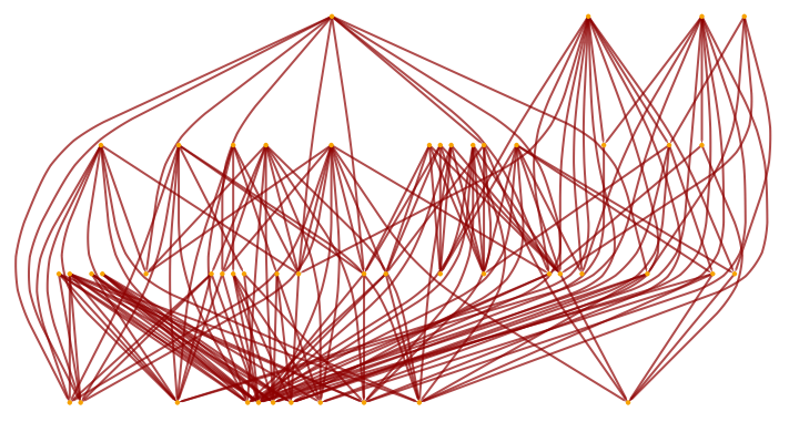
This is a causal graph on a flat spacetime in 3+1 dimensions with 50 causal events sprinkled.
In[]:=
ResourceFunction["CurvedSpacetimeSprinkling"][x^2+y^2,{x,-1,1},{y,-1,1},50]["CausalGraph"]
Out[]=
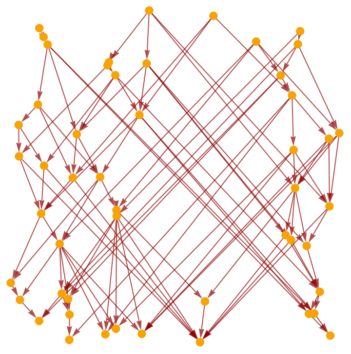
This is a causal graph in 1+1 dimensions with 50 causal events sprinkled on +.With some examples shown, we now ask: which rewriting rules produces a causal graph similar to the above (It is important to note that we are talking about preserving the topology of the graph, rather than taking a look at the location of each node on the sprinkled graphs)? For example, is the topology of the following graph close to the topology of the above causal set?
2
x
2
y
In[]:=
ResourceFunction["WolframModel"][{{x,y},{x,z}}->{{x,z},{x,w},{y,w},{z,w}},Automatic,8,"CausalGraph"]
Out[]=
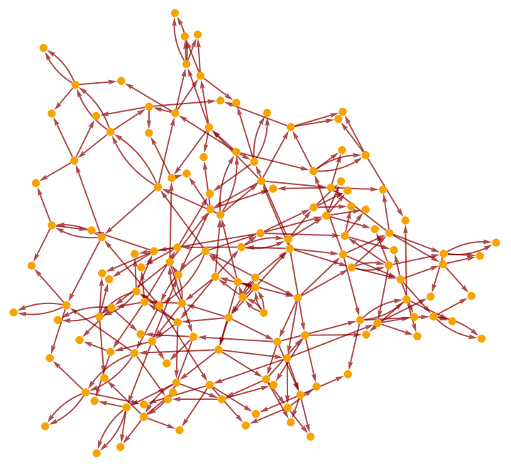
While it looks somewhat similar, we need a mathematical way to determine similarity.
Gauging Differences between Graphs
Gauging Differences between Graphs
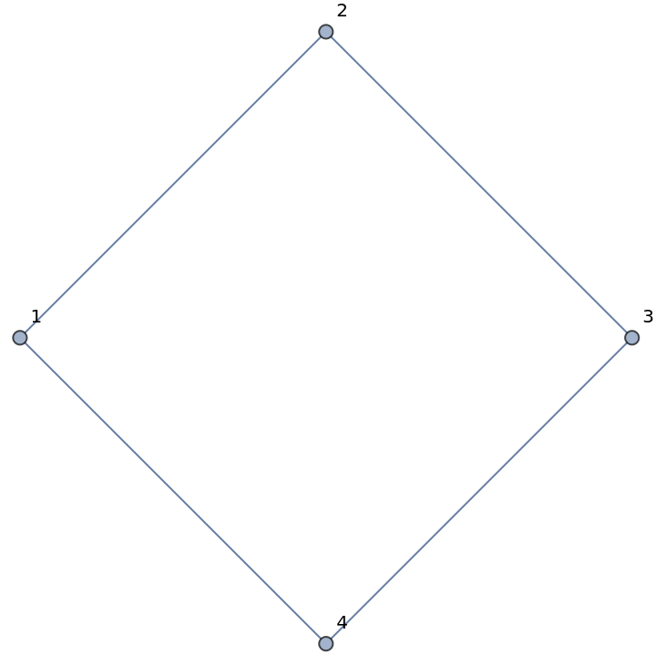
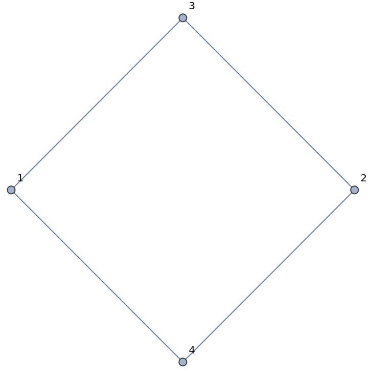
A great place to start is the adjacency matrix of a graph, since it contains information in a format that we are all used to. My initial thought was to subtract the adjacency matrices of two causal graphs and find its Matrix Norm. However, this poses a big problem; this method does not work for isomorphic graphs to begin with (mostly). Of course, if the graph is the exact same, the resulting difference of matrices is the 0 matrix. However, if the vertices are labelled differently, then this method isn’t really viable. For example:
In[]:=
{g,h}={{{0,1,0,1},{1,0,1,0},{0,1,0,1},{1,0,1,0}},{{0,0,1,1},{0,0,1,1},{1,1,0,0},{1,1,0,0}}};MatrixForm/@{g,h}graphs=AdjacencyGraph[#,VertexLabels->Automatic]&/@{g,h}IsomorphicGraphQ@@graphs
Out[]=
,
0 | 1 | 0 | 1 |
1 | 0 | 1 | 0 |
0 | 1 | 0 | 1 |
1 | 0 | 1 | 0 |
0 | 0 | 1 | 1 |
0 | 0 | 1 | 1 |
1 | 1 | 0 | 0 |
1 | 1 | 0 | 0 |
Out[]=
,
Out[]=
True
Notice that these two graphs are isomorphic. However, the norm comes out to be
In[]:=
ResourceFunction["MatrixNorm"][g-h,2]
Out[]=
2.
which is not negligible at all (especially in higher number of nodes). Thus, a better method is needed.
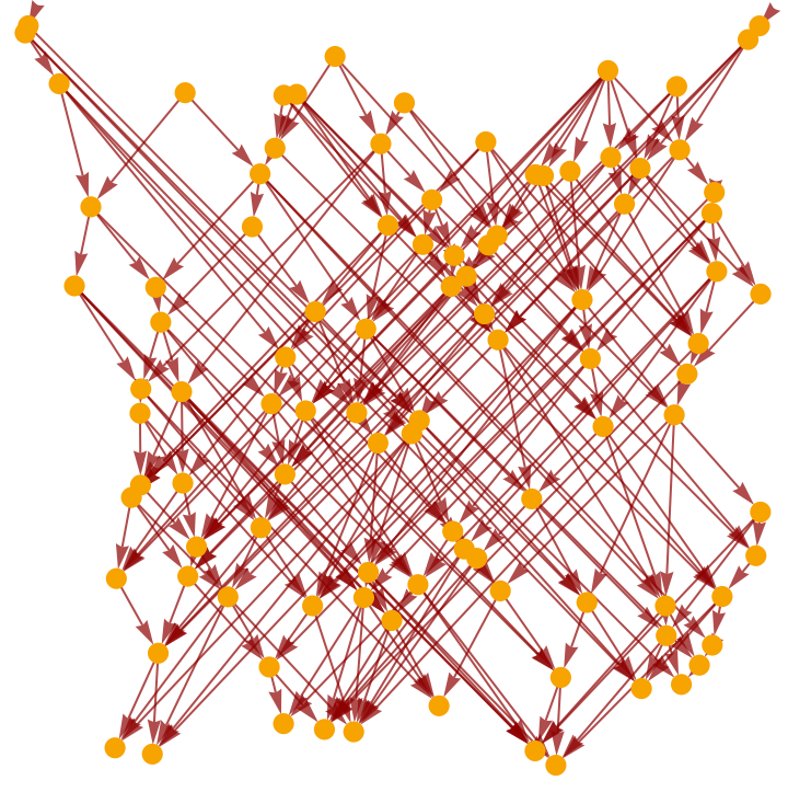
One such method is the spectral adjacency distance, which finds the norm of-, which are the eigenvalues of the adjacency matrices of graphs g and h respectively. A problem with this method is that a lot of causal graphs we find are sparse, resulting in all eigenvalues of 0. This is true for the sprinkled causal graphs as well. For example,
One such method is the spectral adjacency distance, which finds the norm of
g
λ
h
λ
In[]:=
cst=ResourceFunction["FlatSpacetimeSprinkling"][2,100]["CausalGraph"]
Out[]=
In[]:=
Eigenvalues[AdjacencyMatrix[cst]]
Out[]=
{0,0,0,0,0,0,0,0,0,0,0,0,0,0,0,0,0,0,0,0,0,0,0,0,0,0,0,0,0,0,0,0,0,0,0,0,0,0,0,0,0,0,0,0,0,0,0,0,0,0,0,0,0,0,0,0,0,0,0,0,0,0,0,0,0,0,0,0,0,0,0,0,0,0,0,0,0,0,0,0,0,0,0,0,0,0,0,0,0,0,0,0,0,0,0,0,0,0,0,0}
Thus, let us work with Degree Matrices instead. This is just a diagonal matrix with diagonal entries being the degree of a specific node (meaning its eigenvalues are the degrees). Thus, we can compare theses with graphs we create.
Attempts at Rewriting Rules (and their Challenges)
Attempts at Rewriting Rules (and their Challenges)
We first begin with sprinkled graphs on a 1+1 flat spacetime. To determine acceptable error between our graph and a sprinkled one, we can generate two sprinkled graphs and find the error between them. For 100 nodes, we do so with the following code:
In[]:=
dim=100;
In[]:=
cst=ResourceFunction["FlatSpacetimeSprinkling"][2,dim];a=Sort[VertexDegree[cst["CausalGraph"]]];
In[]:=
cst2=ResourceFunction["FlatSpacetimeSprinkling"][2,dim];b=Sort[VertexDegree[cst2["CausalGraph"]]];
In[]:=
sum=0;For[i=1,i<dim+1,i++,sum=sum+(b[[i]]-a[[i]])^2]PrintN[
sum
]dim0.069282
With all of this established, the only thing that remains is finding a rewriting rule that is as close to a sprinkled graph as possible. However, this is a lot easier said than done. One could start with a simple example, like the following:
In[]:=
ex=ResourceFunction["SubstitutionSystemCausalGraph"][{"A"->"ABA","AA"->"BAA","BA"->"AA"},"ABA",3]
Out[]=
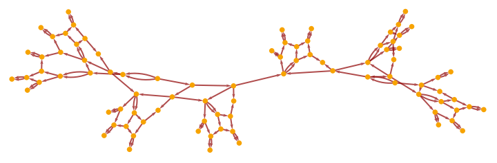
But if we take a look at its degrees (and compare it to the degrees of a sprinkled graph with the same number of nodes), their difference is apparent:
The drastic difference between the maximum degree of each graph is one of the biggest issues we are currently facing. An idea to combat this problem is to create rules such that smaller strings are converted into much larger ones. That way, more rewriting can be done, creating more causal events (which are what nodes represent) as a result. As more nodes are created (and are connected to each other), the degrees of the nodes should be much higher. To test this theory, we try the following example:
Note that the initial conditions and resulting strings of the rewriting rules provide plenty of opportunities for a rule to be used. Now, let us take a look at the degrees of the its nodes, and the degrees of the nodes of a sprinkled causal graph.
Here, we see that maximum of the two lists are comparable (much better than 5 and 13 from the previous example). As such, this ‘technique’ is effective in addressing this first issue. But, is this enough? Let us find the distance between the two graphs:
This is not too bad by all means; however, this value is ~2 times larger than the error between sprinkled graphs. Notice that a big source of error comes from the fact that many more 3’s (that is, small degrees) exist in the first set compared to the second set. Thus, more work is needed to minimize this even further.
Unfortunately, another issue exists. Let us iterate the above example one more time and take a look at its degrees:
Unfortunately, another issue exists. Let us iterate the above example one more time and take a look at its degrees:
One extra iteration adds a tremendous amount of nodes. However, the maximum degree remains pretty much the same! Now, let us check if this is the case for sprinkled graphs. Since the sprinkling of 2700 events requires a lot of computation, we instead use 350 events. Doing so, we assume the reasonable claim that the maximum degree for this setting will be less than or equal to the maximum degree of 2700 nodes.
The difference between 15 and 23 is already large enough to warrant attention. This is especially true considering the fact that this degree should be much higher for 2700 nodes. This increase shows that our above rewriting rule and causal graph don’t capture the time evolution displayed by causal graphs present in Causal Set Theory.
More time and attempts at rewriting rules are needed to come up with a strategy to bypass the two problems posed above.
More time and attempts at rewriting rules are needed to come up with a strategy to bypass the two problems posed above.
Conclusion
Conclusion
Like stated before, we hope to find rewriting rules for CST, which need to address the challenges brought up in the previous section. Once/if we find one rule, we will start looking at systematic ways to find other such rules. Another possibility is looking at causal graphs from hypergraph evolutions instead of strings.
After the 1+1 flat spacetime case, we will move onto curved spacetimes and higher dimension. Then, we plan on moving onto Causal Dynamical Triangulation, another theory of quantum gravity.
After the 1+1 flat spacetime case, we will move onto curved spacetimes and higher dimension. Then, we plan on moving onto Causal Dynamical Triangulation, another theory of quantum gravity.
Acknowledgements
Acknowledgements
I would like to thank Dr. Xerxes Arsiwalla and Eric James Parfitt for their mentoring and guidance the last 10 days. Their help has allowed me to understand this project significantly better (especially the discrete structures and tools available in Mathematica).
CITE THIS NOTEBOOK
CITE THIS NOTEBOOK
Comparing Causal Graphs Between String Rewriting and Poisson Sprinkling in Spacetime
by Anish Suresh
Wolfram Community, STAFF PICKS, January 11, 2024
https://community.wolfram.com/groups/-/m/t/3100485
by Anish Suresh
Wolfram Community, STAFF PICKS, January 11, 2024
https://community.wolfram.com/groups/-/m/t/3100485