This notebook series is designed to introduce selected dynamic economic models to both advanced undergraduate and graduate students. Economists have relied on a series of economic models to better understand the otherwise highly complex causal relationship among many economic variables. Dynamic economic models set up by systems of either difference or differential equations are particularly useful in tracing the change in the quantity of unknown economic variables (e.g., the capital stock, demand for labor, aggregate output, etc.) and their interactions over time.
This notebook series aims to help students better understand the depth, usefulness, and limitations of major existing micro and macroeconomic models by demonstrating how we can use Wolfram Mathematica to replicate and reconstruct the core ideas and find dynamic solution of the model.
The model introduced in this notebook series include, among others, (1) the cobweb model of the quantity and price adjustment, (2) Keynes’s aggregate demand model, (3) Hicks’s ISLM model, (4) Samuelson’s investment accelerator model, (5) Kalecki’s investment delay model, (6) the predator-prey interaction model, (7) the epidemic model, (8) Ricardo’s three dimensional business cycle model, (9) Marx-Goodwin business cycle and growth model, (10) Smith’s and Ricardo’s growth model, (11) the Harrod-Domar growth model, (12) the Solow growth model, (13) the RBC model, (14) Romer’s new growth model, and (15) the circuit of capital model.
The ISLM model with the capital stock and the government’s debt stock accumulation
Introduction
Introduction
Just as in Keynes’s AD models, we have private business investment spending variable in the ISLM model. The difference in these two models is that private business investment in the ISLM model is no longer a fixed quantity, but instead it changes over time depending on both the change in aggregate output-income and the rate of interest. This changing private business investment flow will affect the trajectory of the accumulation process of the productive capital stock.
Just as we did in Keynes’s AD model, we can also introduce the government sector in the ISLM model, in which the government imposes a marginal tax rate regime on gross income, while engaging in a certain fixed expenditure (both government spending and income transfer). If the government’s spending is greater than its revenue at a given point in time (called ‘primary deficit’), it will be recorded and accumulated as the government’s debt stock over time.
This note extends the baseline ISLM model to account for these two important stock variables, both the capital stock and the government’s debt stock. From a mathematical point of view, the capital stock is an integral of the variable private business investment spending. The same is true for the government’s debt stock; it is an integral of the government’s fiscal deficit. In this note, we demonstrate how we can use both difference equation and differential equation to simulate the capital stock and debt stock accumulation process.
A difference equation model
A difference equation model
The derivation of the model and its analytical solution
The derivation of the model and its analytical solution
Recall that the original ISLM model consists of the following two linear equations:
Y=a+bY+PBI(a,b>0)kY-hR=M(k,h>0)
(
1
)where PBI = CBI + cY - dR (c, d > 0).
The parameter a is an autonomous consumption spending, b is the marginal propensity to consume as in Keynes’s AD models. Private business investment spending consists of the following three components: CBI represents constant business investment spending, which is necessary to maintain a portion of the existing capital stock as before, c is an output sensitivity of investment spending, and d is an interest rate sensitivity of investment spending. In this formulation, private business investment spending is assumed to be a positive function of aggregate output-income (Y) and a negative function of the rate of interest (R). Both k and h are output sensitivity and interest rate sensitivity of money demand.
If we introduce the government sector assuming that the government imposes a marginal tax rate regime, we can modify the previous linear system in (1) into the following linear first-order difference equation for the change in aggregate output-income:
Y[t]=a+b*(Y[t-1]-τY[t-1]+TR)+PBI[t]+G(a,b>0)
(
2
)where τ is the average marginal tax rate on gross income, TR is the transfer income granted to selected households, and G is a fixed government expenditure. In this formulation, we assume that households’ current consumption spending is determined by their disposable income measured at one time period earlier.
Notice that PBI[t] is no longer a fixed quantity, and therefore we need to specify this variable further. For simplicity, let us suppose that the current private business investment spending, PBI[t], is affected by the current value of aggregate output-income (Y[t] and the rate of interest at the same period (R[t]). If we further assume that the rate of interest at time t, R[t], is also a function of aggregate output-income at the same period (Y[t]) given money supply, then we can define the following functional definition of both PBI[t] and R[t]:
R[t]=(kY[t]-M)/h(k,h>0)PBI[t]=CBI+c*Y[t]-d*R[t](c,d>0)
(
3
)For our later computational ease, let us define a function of these two variables as follows:
In[]:=
Clear[a,b,c,d,τ,G,TR,Y,R,PBI,CBI,k,h,M,Y0,t,sol];PBI[t_]:=CBI+c*Y[t]-d*R[t];R[t_]:=(kY[t]-M)/h;
The analytical solution to the linear first-order difference equation for Y[t] in (2) appear in these two functions of PBI[t] and R[t]. Therefore, we need to find the general solution to the difference equation for Y[t] and substitute the solution into both PBI[t] and R[t] in (3).
First, the solution to Y[t] is:
In[]:=
sol=RSolve[{Y[t]==a+b*(Y[t-1]-τY[t-1]+TR)+PBI[t]+G,Y[0]==Y0},Y[t],t]//Simplify
Out[]=
Y[t]Gh+dM+bhTR-ah-1+-CBIh-1+-Gh-dM-bhTR+hY0-bhY0-chY0+dkY0+bhY0τ
1
dk-h(-1+b+c-bτ)
t
bh(-1+τ)
(-1+c)h-dk
t
bh(-1+τ)
(-1+c)h-dk
t
bh(-1+τ)
(-1+c)h-dk
t
bh(-1+τ)
(-1+c)h-dk
t
bh(-1+τ)
(-1+c)h-dk
t
bh(-1+τ)
(-1+c)h-dk
t
bh(-1+τ)
(-1+c)h-dk
t
bh(-1+τ)
(-1+c)h-dk
t
bh(-1+τ)
(-1+c)h-dk
t
bh(-1+τ)
(-1+c)h-dk
Next, substituting this Y[t] solution into (3) to get a more detailed expression for both PBI[t] and R[t], we get:
In[]:=
PBI[t]/.solR[t]/.sol
Out[]=
CBI+cGh+dM+bhTR-ah-1+-CBIh-1+-Gh-dM-bhTR+hY0-bhY0-chY0+dkY0+bhY0τ-d-M+kGh+dM+bhTR-ah-1+-CBIh-1+-Gh-dM-bhTR+hY0-bhY0-chY0+dkY0+bhY0τ
1
dk-h(-1+b+c-bτ)
t
bh(-1+τ)
(-1+c)h-dk
t
bh(-1+τ)
(-1+c)h-dk
t
bh(-1+τ)
(-1+c)h-dk
t
bh(-1+τ)
(-1+c)h-dk
t
bh(-1+τ)
(-1+c)h-dk
t
bh(-1+τ)
(-1+c)h-dk
t
bh(-1+τ)
(-1+c)h-dk
t
bh(-1+τ)
(-1+c)h-dk
t
bh(-1+τ)
(-1+c)h-dk
t
bh(-1+τ)
(-1+c)h-dk
1
h
1
dk-h(-1+b+c-bτ)
t
bh(-1+τ)
(-1+c)h-dk
t
bh(-1+τ)
(-1+c)h-dk
t
bh(-1+τ)
(-1+c)h-dk
t
bh(-1+τ)
(-1+c)h-dk
t
bh(-1+τ)
(-1+c)h-dk
t
bh(-1+τ)
(-1+c)h-dk
t
bh(-1+τ)
(-1+c)h-dk
t
bh(-1+τ)
(-1+c)h-dk
t
bh(-1+τ)
(-1+c)h-dk
t
bh(-1+τ)
(-1+c)h-dk
Out[]=
-M+kGh+dM+bhTR-ah-1+-CBIh-1+-Gh-dM-bhTR+hY0-bhY0-chY0+dkY0+bhY0τ
1
h
1
dk-h(-1+b+c-bτ)
t
bh(-1+τ)
(-1+c)h-dk
t
bh(-1+τ)
(-1+c)h-dk
t
bh(-1+τ)
(-1+c)h-dk
t
bh(-1+τ)
(-1+c)h-dk
t
bh(-1+τ)
(-1+c)h-dk
t
bh(-1+τ)
(-1+c)h-dk
t
bh(-1+τ)
(-1+c)h-dk
t
bh(-1+τ)
(-1+c)h-dk
t
bh(-1+τ)
(-1+c)h-dk
t
bh(-1+τ)
(-1+c)h-dk
The definition of the three relevant functions
The definition of the three relevant functions
The specification of both the capital stock and debt accumulation
The specification of both the capital stock and debt accumulation
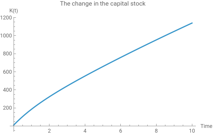
The productive capital stock in this model economy accumulates as the variable quantity of private business investment spending is positive. If we assume that there is a constant depreciation rate, δ, the capital stock at time t can be defined as:
K[t]=K[t-1]+PBI[t]-δK[t]
(
4
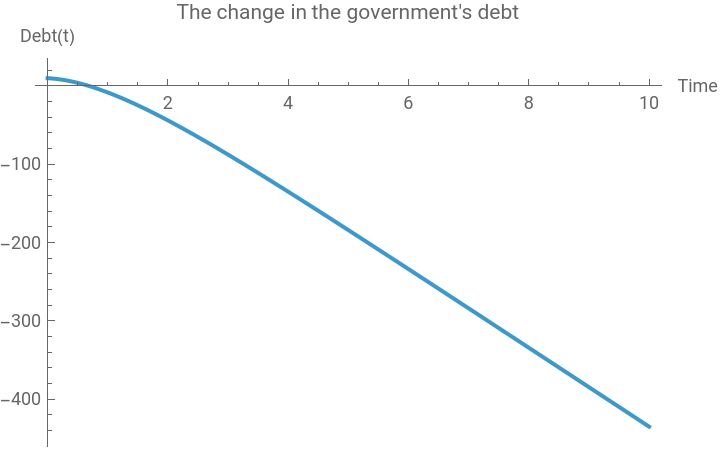
)Similarly, if the sum of the two government spending flows, G + TR, is greater than the government’s tax revenue, τY, the government sector will accumulate its debt as follows:
Debt[t]Debt[t-1]+(G+TR)-τY[t]
(
5
)Notice that the capital stock accumulation is an integral of the changing private business investment spending that is affected by both Y[t] and R[t]; similarly, the government’s debt is also affected by the changing aggregate output-income and its two fixed spending components.
The simulation with fixed parameters and initial conditions
The simulation with fixed parameters and initial conditions
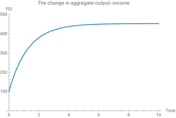
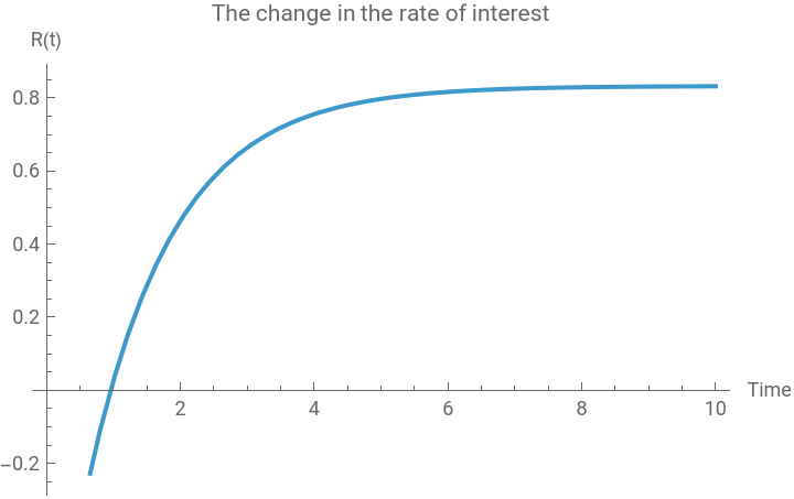
For more concrete understanding, let us introduce the following arbitrary numerical values to parameters and initial values. The numerical solution will be:
In[]:=
Clear[a,b,c,d,k,h,M,δ,τ,K,K0,Debt,Debt0,t,eqn1,sol1];a=10;b=0.8;c=0.6;d=200;τ=0.2;δ=0.02;k=3.5;h=700;M=1000;CBI=10;G=30;TR=10;Y0=100;K0=10;Debt0=10;eqn1={K[t]K[t-1]+PBI[t]-δK[t],Debt[t]Debt[t-1]+(G+TR)-τY[t],K[0]==K0,Debt[0]==Debt0};sol1=RSolve[eqn1,{K[t],Debt[t]},t][[1]];Plot[Y[t],{t,0,10},PlotRange->{0,500},PlotLabel->"The change in aggregate output-income",AxesLabel->{"Time","Y(t)"}]Plot[R[t],{t,0,10},PlotRange->Automatic,PlotLabel->"The change in the rate of interest",AxesLabel->{"Time","R(t)"}]Plot[K[t]/.sol1,{t,0,10},PlotRange->Automatic,PlotLabel->"The change in the capital stock",AxesLabel->{"Time","K(t)"}]Plot[Debt[t]/.sol1,{t,0,10},PlotRange->Automatic,PlotLabel->"The change in the government's debt",AxesLabel->{"Time","Debt(t)"}]
Out[]=
Out[]=
Out[]=
Out[]=
A differential equation model
A differential equation model
The derivation of the model and its analytical solution
The derivation of the model and its analytical solution
The same idea can be formulated by a continuous time model. Suppose that at each period excess demand in both product market and money market is adjusted by a certain parameter, α and β. The differential equation formulation can be written as:
where PBI[t] = CBI + cY[t] - dR[t] (c,d >0).
This is a system of two linear first-order non-homogenous differential equations, whose symbolic solutions can be found by:
The specification of both the capital stock and debt accumulation
The specification of both the capital stock and debt accumulation
The productive capital stock will accumulate as firms engage in private business investment spending as follows:
The government’s debt stock will also accumulate as follows:
The simulation with fixed parameters and initial conditions
The simulation with fixed parameters and initial conditions
Suppose we have the following arbitrary numerical values to parameters and initial values:
An interactive visualization
An interactive visualization
One beauty of using Wolfram Mathematica is that it allows us to create an interactive graph that shows us how the solution curve changes if there is any change in relevant parameters and the initial value that constitute the model. As a last step of our analysis of the ISLM model, let us examine the following syntax and the interactive graphical solution:
Conclusion
Conclusion
In this note, we have sought to extend the previous dynamic ISLM model to account for the accumulation of both capital stock and the government debt stock. The solution to both aggregate output-income and the rate of interest equation determines the volume of private business investment spending, which then affect the trajectory of the accumulation of the productive capital stock. The solution to aggregate output-income equation gives rise to a unique value of the government’s fiscal balance, which affect the trajectory of the possible accumulation of the government’s debt stock over time.
One may want to extend this macroeconomic model to account for selected labor market variables. For example, if we assume that there is a fixed capital-labor ratio, we can determine the changing value of labor demand as the productive capital stock is accumulated in this model economy. If we further assume a constant growth rate of labor force, we can also determine the level of employment and unemployment, both of which will give us the rate of unemployment.
Reference
Reference
John Hicks, “Mr. Keynes and the “Classics” - A Suggested Interpretation,” Econometrica, Vol. 5, No. 2 (April 1937), pp.147-159.
--------------, “IS-LM: An Explanation,” Journal of Post Keynesian Economics, Vol. 3, No. 2 (1980-1981), pp.139-154.
John M. Keynes, The General Theory of Employment, Money and Interest. New York: Prometheus Books, 1997 [1936].
Ronald Shone, An Introduction to Economic Dynamics, Cambridge University Press: 2001, pp.91-109.
Ronald Shone, Economic Dynamics, Cambridge University Press: 1997, pp.265-308.
Srinivas Raghavendra and Petri T. Piiroinen, An Introduction to Economic Dynamics - Modelling, Analysis and Simulation, Routledge: 2023, pp.61-78.
CITE THIS NOTEBOOK
CITE THIS NOTEBOOK
Introduction to dynamic economic models: The ISLM model with the capital stock and debt
by Hee-Young Shin
Wolfram Community, STAFF PICKS, December 14, 2025
https://community.wolfram.com/groups/-/m/t/3590761
by Hee-Young Shin
Wolfram Community, STAFF PICKS, December 14, 2025
https://community.wolfram.com/groups/-/m/t/3590761