Introduction
In flat space, the shortest distance between two points is a straight line. But what about finding the distance between two points in curved surfaces, wether it is a sphere or a saddle or even a torus? Generalized straight lined paths are called geodesics and are important in GPS systems, virtual reality, and many other 3D landscapes, which is where my first interest and ideas began. This project will explore geodesics in multiple scenarios: first from 2D planes, to spherical shapes such as a planet, hyperbolic disks, variable-curvature surfaces, and a torus. This project will also concentrate on visualizations of geodesics paths on a torus, or also known as toroidal geometry.
Euclidean Geodesics on a 2D Plane
In[]:=
point1={0,0};point2={3,2};euclideanDistance=Norm[point2-point1]; Graphics[{Red,PointSize[Large],Point[point1],Blue,Point[point2],Black,Line[{point1,point2}]}]Print["The euclidean distance between point 1(0,0) and point 2(3,2) is: ",euclideanDistance];
Out[]=
The euclidean distance between point 1(0,0) and point 2(3,2) is:
13
The code above shows two points, p1 and p2, on a 2D plane. The definition of ‘euclideanDistance’ on the third line uses a function, ‘Norm’, to calculate the distance between the two points. This is similar to as if we just used the distance formula. Then, I used ‘Graphics’ to draw the points and the line for better visualization.
Spherical Geodesic Routes on Earth
In[]:=
NYC=Entity["City",{"NewYork","NewYork","UnitedStates"}];PAR=Entity["City",{"Paris","IleDeFrance","France"}];path=GeoPath[{NYC,PAR}];distance=GeoDistance[NYC,PAR];GraphicsRow[{GeoGraphics[{Red,PointSize[Medium],Point[NYC],Blue,Point[PAR],Thick,path}]}]Print["The distance from NYC to PAR is ",ToString[UnitConvert[distance,"Miles"]]]
Out[]=
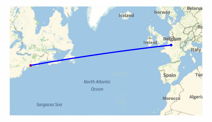
The distance from NYC to PAR is 3613.99 miles
For this block of code, I first defined two cities, ‘NYC’ and ‘PAR’ using ‘Entity’, which allows me o define specific properties for these cities, in this case, to make it easier to find geographic paths and distances. The ‘path’ variables find the route between these two cities on a map, while ‘distance’ finds the length of the route from one city to another. Then, using ‘GeoGraphics’, I visualized the line on the map. The output shows the distance from New York City to Paris in miles. One thing to note is that this is the fastest path form New York City to Paris. The line may seem to be straight, but if it were to be put on a curved surface, such as an image of planet Earth, it would appear to look curved. This shows that the fastest distance to travel from one place to another on a 3D sphere may not be a straight line. This is specifically used in airline flights, where planes take a curved route most of the times instead of a straight line since it is faster, but that is a whole different topic for another time.
Hyperbolic Geodesics on the Poincare Disk
In[]:=
poincarePoints={{-0.5,-0.3},{0.5,0.2}};GeodesicCurve[p1_,p2_]:=Module[{middle,direction,perpDirection,center,radius,startAngle,endAngle},middle=(p1+p2)/2;direction=Normalize[p2-p1];perpDirection={-direction[[2]],direction[[1]]};center=middle+0.4*perpDirection;radius=Norm[p1-center];startAngle=ArcTan@@(p1-center);endAngle=ArcTan@@(p2-center);Circle[center,radius,{startAngle,endAngle}]]curve=GeodesicCurve@@poincarePoints;Graphics[{LightGray,Disk[],Blue,PointSize[Large],Point/@poincarePoints,Red,Thick,curve}]
Out[]=
For this block of code, there are two points that are chosen within the disk to show what hyperbolic space in non-euclidean geometry looks like. The ‘poincarePoints’ and the ‘GeodesicCurve’ functions find the euclidean circle, which is the arc that you see above. It first finds the midpoint between the two given points and the direction vector from one point to another. Then, it rotates the direction by ninety degrees to find a perpendicular vector. This new vector is used to find the center of the circle. The radius of the circle is essentially the distance from the center to one of the points. The arc is drawn using the ‘Circle” object. The ‘startAngle’ and ‘endAngle’ define the angular position from the center of the circle to the two points. Then, using the ‘Graphics’ object, the full image is shown. This image shows a hyperbolic geodesic, which appears as an arc that intersect the boundary of a disk at a ninety degree angle.
Numerical Geodesics on Curved Surfaces
In[]:=
f[x_,y_]:=0.2 x^2-0.2 y^2X[x_,y_]:={x,y,f[x,y]}derivU=D[X[x,y],x];derivV=D[X[x,y],y];dotProductUU=derivU.derivU;dotProductUV=derivU.derivV;dotProductVV=derivV.derivV;metric={{dotProductUU,dotProductUV},{dotProductUV,dotProductVV}};metricInverse=Simplify[Inverse[metric]];coords={x,y};gamma=Table[Sum[1/2 metricInverse[[i,k]]*(D[metric[[k,j]],coords[[l]]]+D[metric[[k,l]],coords[[j]]]-D[metric[[j,l]],coords[[k]]]),{k,1,2}],{i,1,2},{j,1,2},{l,1,2}];geodesicEquations={x''[s]+(gamma[[1,1,1]]/. {x->x[s],y->y[s]})*x'[s]^2+2*(gamma[[1,1,2]]/. {x->x[s],y->y[s]})*x'[s]*y'[s]+(gamma[[1,2,2]]/. {x->x[s],y->y[s]})*y'[s]^2==0,y''[s]+(gamma[[2,1,1]]/. {x->x[s],y->y[s]})*x'[s]^2+2*(gamma[[2,1,2]]/. {x->x[s],y->y[s]})*x'[s]*y'[s]+(gamma[[2,2,2]]/. {x->x[s],y->y[s]})*y'[s]^2==0,x[0]==0.5,y[0]==0.2,x'[0]==0.6,y'[0]==0.3};ParametricPlot[Evaluate[{x[s],y[s]}/. NDSolve[geodesicEquations,{x,y},{s,0,10}]],{s,0,10},PlotRange->All,AxesLabel->{"x","y"},PlotStyle->{Thick,Blue}]
Out[]=
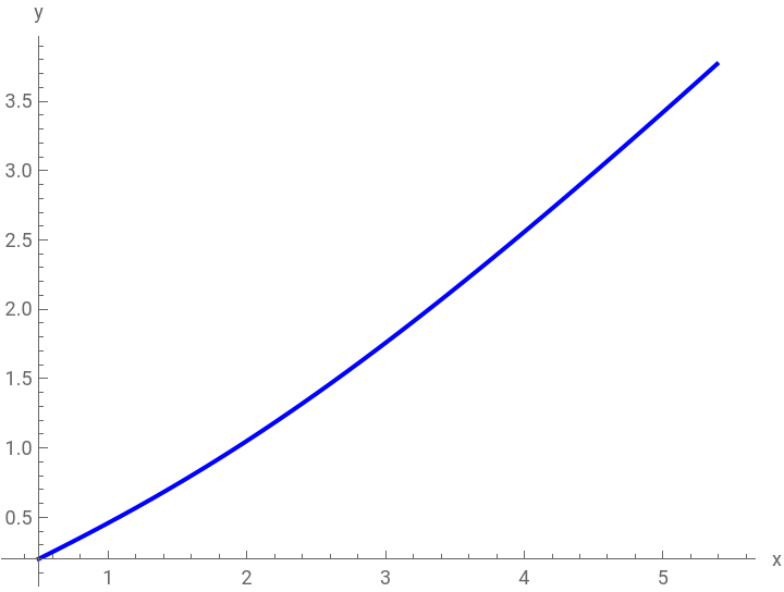
In this code, the first line defines the shape of the saddle surface, which would look like an upward curve in the x-direction and a downward curve in the y-direction. Then the second line is an embedding of 2D coordinates into a 3D space by mapping each point in which z is a function of x and y. Then, I am able to find the tangent vector for both the x-direction and the y-direction by finding the partial derivative of the surface with respect to x an the partial derivative with respect to y. I will use these tangent vectors to find the dot products. Using these dot products, I can construct the several components of the metric tensor. For those who are confused on what a metric tensor is, it is an object that describes the geometry of a shape, such as how distances and the angles are measured. These derivatives build up ‘metric’, a two by two matrix that tells us how to measure distance and angles on a curved surface. ‘metricInverse’ takes the inverse of this matrix to find the Christoffel symbol, which is am object to describe how the surface curves. Then comes ‘gamma’, which I defined to locate all possible Christoffel symbols using derivatives of the metric and the inverse. Using the formula shown below, we can find that there will be a total of 8 Christoffel symbols for a 2D surface. I must say that I could not find any other image online of this formula with the correct symbols, so I apologize for the inconvenience. I will correct them below:-Instead of lambda(denoted as a upside down y), I used ‘i’ -Instead of mu(denoted as u), I used ‘j’ -Instead of nu(denoted as v), I used ‘k’ -Instead of alpha(denoted as a), I used ‘l’ Then, ‘geodesicEquations’ then defines a system of second-order differential equations to describe geodesics, specifically that they minimize the distance on curved surfaces. These equations are formed from the second derivative of ‘s’, which will be acceleration, the first derivatives of ‘s’, which is velocity, and the Christoffel symbols. Using all this information, I am finally able to plot the 2D parametric plot of the geodesic path using ‘ParametricPlot’. Instead of drawing it on a 3D surface, since the motion happens there, I decided to use 2D to better understand the shape it of its domain.

Side-by-Side Comparisons
This cell block compares how geodesics look like in the four types of geometries we looked at in this project. We looked at Euclidean, spherical, hyperbolic, and numerical, which is the on about the saddle. For the code, I just combined all previous blocks into one table, where each panel has the graph or table and the name. By looking at the graphs side by side, we can see that flat geometry shows straight lines, spherical geometry shows paths that are curved outwards, and hyperbolic and saddle geometry shows an intricate response to curves.
Comparing and Understanding the Distances of Each Geodesic
The following code print out the different types of distances in different geometric shapes. The code first generates a geodesic path via solving a differential equation, which is found under ‘NDSolve’, and then find five different lengths. The Euclidean distance at 3.60555, or the square root of thirteen, is measured by taking the distance between (0,0) and (3,2) on a flat 2D plane. The spherical distance at 5816.15 kilometers is found by the shortest, which is not necessarily a straight line but rather a curve, between New York City and Paris along the surface of the planet. For the hyperbolic length, at around 2.53296, I used the Poincare disk model to find an arc inside the gray disk and measure the distance. For the saddle length, 6.07397 is the true shortest path on the 3D saddle, which was the numerical graph mentioned before. Each of the results are rounded to five decimal place accuracy, and the sphere distance is measured in kilometers due to the physical distance between New York City and Paris whereas the other results do not have a set unit measurement.
Visualizing the Shortest Path on a Torus
This code introduces a torus, specifically about finding the shortest path on a torus’s surface. First we defined parameters R and r. The next part of the code is written to create a parametric equation for a torus using ‘u’ and ‘v’, where the outputs are (x,y, z) coordinates for any (u,v) point on the torus. After this, I compute the partial derivative to get tangent vectors. Using these vectors I can build the metric tensor(mentioned earlier) by dotting the tangent vectors to measure how distances and angles are distorted on the curved surface. Te ‘metricInverse’ inverts the metric tensor and the ‘GammaTorus’ finds the Christoffel symbol the encodes how vectors change when moved along the surface. Then, ‘geodesicTorus’ solves for ‘u(s)’ and ‘v(s)’ with the initial position and velocity, and then the 3D solution is printed out, which is a geodesic curve winded around the torus’s surface.
3D Torus Visualization with Geodesic Paths
This part of the project looks at generating geodesic curves from a single starting point on a surface of a torus. First, the torus is defined via ‘R=1’ as the major radius, and ‘r=0.4’ as the minor radius. Using the functions ‘X[u,v]’, I was able to convert both the parameters, ‘u’ and ‘v’, into 3D coordinates. The starting point for all geodesics is at the very center of the torus’s tube, where ‘u0’ is zero and ‘v0’ is pi/2. The ‘angles’ array divides the whole circle into seven equal parts spaced around the torus in order to represent an initial velocity for each geodesic. Then, for each specific angle, I use differential equation, which is done by using ‘NDSolve’, to find how the geodesic moves around the surface of the torus. Then this is all plotted using ‘ParametricPlot3D’, which gives a color from the rainbow to each line to distinguish each line from the other. I will acknowledge though, that at first glance it does look somewhat messy. I have marked the starting point of all lines with a giant red dot so it is easier to find . ‘Show’ then combines all of the 3D visualizations into one.
Conclusion
This project on geodesics looked at the differences in shortest-path geometry across different surfaces, such as Euclidean, spherical, hyperbolic, and curved surfaces. By solving geodesics equation, this project showed how curvature affects path lengths and trajectories, where the straight lines show shorter distances, while the curved paths show longer distances because of the natural shape of the objects. The torus geodesic showed how surface topology creates complex, and somewhat weird trajectories that are impossible in flat, Euclidean geometry. These results conform with the standards of geometry while also showing examples of abstract mathematical concepts.
Applications
This project has many different applications in several fields. For example, in physics these methods could help predict particle motion in curved space for gravitational wave applications. On the other hand, engineers could use them to optimize robotic paths across curved and uneven terrain. Furthermore, the mapping algorithms for map applications can enhance GPS navigation by better accounting for the shape of the planet, with its uneven terrain. Of course there are a bunch of other applications that can be used, but these are the ones that came straight to my mind and are the most important. There are a lot of other applications where using geometric curvature can help solve real-world pathing problems.
Future Works
From this project, there could be many possible works that could emerge. One of the possible branches from this project is looking at higher-dimensional surfaces such as Klein bottles, which is a one-sided surface which, if traveled upon, could be followed back to the point of origin while flipping the traveler upside down. This section of this project could potentially look at new topological constraints on geodesic behaviors. Another possible idea is potentially developing a machine learning surrogate model to predict geodesics, which could reduce computational time and can be applied in real-time applications, possibly in autonomous vehicles. Another idea is to investigate how geodesic networks form properties in transportation infrastructure or quantum gravity models, which could lead to some interesting results. Each possible branch from this project can build on this project and expand on the topic of geodesics.
Keywords
-Geodesics
-Geometry
-2D Plane
-3D Plane
-Sphere
-Poincare Disk
-Curved Surface
-Saddle Surface
-Torus
-Geometry
-2D Plane
-3D Plane
-Sphere
-Poincare Disk
-Curved Surface
-Saddle Surface
-Torus