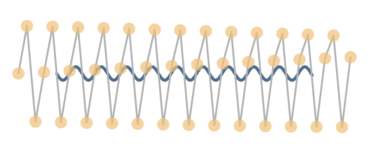
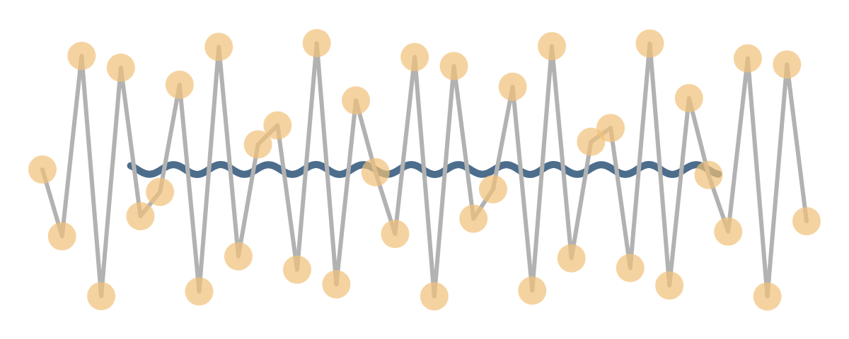
Two waves, one gray and one blue, are moving synchronously. In appearance, the blue wave moves in a simple, predictable pattern that perhaps does not inspire much interest. The gray one, is both fancier in both appearance, with its accented yellow dots, and wilder in behavior. It starts out in a similar fashion, then the yellow dots starts forming some dramatic, waving pattern. Suddenly chaos ensue as my mind strain to observe the pattern of the dancing yellow dots. Yet before I can catch on, these dots are back at their symmetric choreography. Another brief burst of chaos, and then the paths gradually merge for the next loop.
I wanted to test how many Dynamic primitives my 5 years old laptop can handle in one scene (i.e. Graphics). It was my first test scenario:
In[]:=
With{num=40,aspRatio=3,splineOrder=10},With{freqSet=Rescale@Range@num},DynamicModule{t=0,pts=Thread[{Rescale[Range[num],{1,num},aspRatio{-1,1}],0}]},DynamicWrapperGraphics[{{CapForm@"Round",Hue[0.58,0.45,0.55],AbsoluteThickness@5,BSplineCurve[Dynamic@pts,SplineDegree->splineOrder,SplineKnots->"Unclamped"]},{CapForm@"Round",JoinForm@"Round",GrayLevel@0.7,AbsoluteThickness@3,Line@Dynamic@pts},{Hue[0.1,0.5,0.95,0.7],AbsolutePointSize@20,Point@Dynamic@pts}},PlotRange->{aspRatio{-1,1},{-1.2,1.2}},PlotRangePadding->Scaled[0.05],ImageSize->600],t=Clock0,39,;pts=MapIndexed[Function[{f,idx},{Rescale[idx〚1〛,{1,num},aspRatio{-1,1}],Sin[2πft]}],freqSet]
1
60
Out[]=
Not too shabby! The motions are smooth, the points align perfectly. The performance of the FrontEnd is impressive!
Additionally, I want to write down some technical details here. They were interesting but didn’t fit into the original post.
Note that each yellow point has a unique frequency , which linearly increases from 0 at the left most to 1 at the right most. They start synchronously at time mark , thus the whole group return to its starting state for the first time at , where
f
t=0
t=T
T:=LCM( T 2 T k T n |
=LCM( -1 f 2 -1 f k -1 f n |
=LCM -1 2-1 n-1 -1 k-1 n-1 -1 n-1 n-1 |
=n-1 |
For the animation above, it’s .
T=40-1=39
During the runtime of the animation, several spirals emerge from “chaos” from time to time. It’s a result of points align with neighbors at different distances away. The pattern is easily spotted in the following graphic at :
y=T(i,k∈)
i
k
Module{num=40,T},T=num-1;alignments=Functionk,T,RawBoxes@RowBox[{FractionBox[#,k],"T"}]&/@Range[k-1]/@{2,3,4,5,6}//Apply@Join//GroupBy[First->Last]//Map@First//KeyValueMap[List];Range[T+1]//Rescale//Sin[2π#t]&//(Through@*{##}&)Plot#,t,0,1.01,FrameTicks->{{None,None},{Range[0,T],alignments}},&,Plot#,t,0.99,T,FrameTicks->{{None,None},{alignments,Range[0,T]}},&//Column[#,Spacings->1]&
#
k
T
2
T
2
Out[]=


When doing discrete uniform sampling at a right sampling rate:
In[]:=
Range[40]//Rescale//Sin[2π#t]&//DiscretePlot#,t,0,,,FrameTicks->{{None,None},{Range[0,39],alignments}},&
39
2
39
LCM@@Range[6]
Out[]=

or we can plot with the states slightly before and after the above sampling time marks to see the difference between T and T:
i
2k
i
2k+1
In[]:=
Withtgrid=#+.1{-1,0,1}&/@Range0,,//Flatten,Range[40]//Rescale//Sin[2π#t]&//DiscretePlot#,{t,tgrid},FrameTicks->{{None,None},{Range[0,39],alignments}},&
39
2
39
60
Out[]=

Taking a close look at each time the dots’ waves rising:
In[]:=
Withnum=40,aspRatio=3,splineOrder=10,kset=Functionk,&/@Range[k-1]/@{2,3,4,5,6}//Flatten[{0,#,1}]&//Union,With[{freqSet=Rescale@Range@num},DynamicModule[{k=0,Δt=0,t=0,pts},pts=MapIndexed[Function[{freq,idx},{Rescale[idx〚1〛,{1,num},aspRatio{-1,1}],Sin[2πfreqt]}],freqSet];Column[{Grid[{RadioButtonBar[Dynamic[k,(k=#;Δt=0.;t=39k;pts=MapIndexed[Function[{freq,idx},{Rescale[idx〚1〛,{1,num},aspRatio{-1,1}],Sin[2πfreqt]}],freqSet];)&],Thread[kset->kset"T"]]//{"k",#}&,Slider[Dynamic[Δt,(Δt=#;t=39k+Δt;pts=MapIndexed[Function[{freq,idx},{Rescale[idx〚1〛,{1,num},aspRatio{-1,1}],Sin[2πfreqt]}],freqSet];)&],{-.1,.1,.001},Appearance->"Labeled"]//{"Δt",#}&,{"t",Dynamic[t]}},Alignment->{{Right,Left},Center},Spacings->{2,Automatic}],Graphics[{{CapForm@"Round",Hue[0.58,0.45,0.55],AbsoluteThickness@5,BSplineCurve[Dynamic@pts,SplineDegree->splineOrder,SplineKnots->"Unclamped"]},{CapForm@"Round",JoinForm@"Round",GrayLevel@0.7,AbsoluteThickness@3,Line@Dynamic@pts},{Hue[0.1,0.5,0.95,0.7],AbsolutePointSize@20,Point@Dynamic@pts}},PlotRange->{aspRatio{-1,1},{-1.2,1.2}},PlotRangePadding->Scaled[0.05],ImageSize->600]}]]]
#
k
Out[]=
| ||||||||||||||||||||||||||||||||||