1D PSO on a multi-modal fitness landscape
1D PSO on a multi-modal fitness landscape
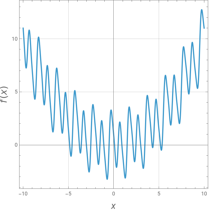
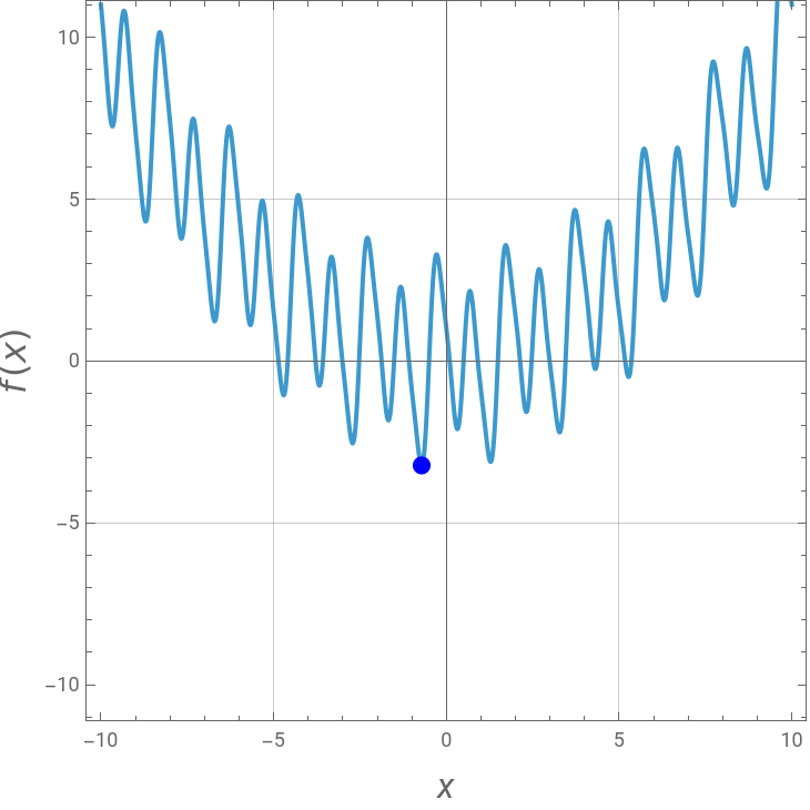
Particle swarm optimization (PSO) comes from the pioneering work of Kennedy and Eberhart[1, 2]. PSO algorithms mimic the social behavior patterns of organisms that live and interact within large groups, such as swarms of bees. This optimization technique is used to find the minimum of the following 1D test function: , with ; you can vary the parameters and (here a and b are set equal to 0.1 and 2, respectively). For the global minimum of (indicated by the blue dot), perfect agreement is found using either the Mathematica built-in command NMinimize or PSO. You can vary the number of iterations as well as the swarm size. However, notice the complementary effect of these parameters. Here, the problem is one-dimensional, but extension to multidimensional problems using the program is straightforward.
f(x)=a+cos(πx)-bsin(2πx)+cos(3πx)sin(πx)
2
x
x∈[-10,10]
a
b
f(x)
1D problem
SwarmDim=1;
Upper and lower bounds for the search domain
FitnessLB=-10;FitnessUB=10;
PSO parameters
c1=2;c2=2;w=0.72984;
a=0.1;b=2;Fitness[{x_}]:=ax^2+Cos[Pix]-bSin[2Pix]+Cos[3Pix]Sin[Pix];;
Plot of the fitness function
plot=Plot[Fitness[x],{x,-10,10},FrameTrue,AspectRatio1,GridLinesAutomatic,FrameLabel{Style["x",16,Italic],Text[Row[{Style["f",16,Italic],Style["(",16],Style["x",16,Italic],Style[")",16]}]]}]
Out[]=
In[]:=
sol=NMinimize[Fitness[x],x,Method"SimulatedAnnealing"][[2]]
Out[]=
{x-0.715369}
PSO Optimizer
psoOptimize[lossFunc_,dim_,lb_,ub_,nParticles_:150,nIter_:80,w_:0.72984,c1_:2,c2_:2]:=Module[{particles,velocities,pbest,pbestScore,gbest,gbestScore,convergence={},r1,r2,score,gbestIdx},(*Initializeparticlesuniformlywithin[lb,ub]ineachdimension*)particles=RandomReal[{lb,ub},{nParticles,dim}];velocities=ConstantArray[0.,{nParticles,dim}];pbest=particles;pbestScore=Table[lossFunc[particles[[i]]],{i,nParticles}];gbestIdx=First@Ordering[pbestScore,1];gbestScore=pbestScore[[gbestIdx]];gbest=pbest[[gbestIdx]];Do[Do[r1=RandomReal[1,dim];r2=RandomReal[1,dim];velocities[[i]]=w*velocities[[i]]+c1*r1*(pbest[[i]]-particles[[i]])+c2*r2*(gbest-particles[[i]]);particles[[i]]+=velocities[[i]];(*keepparticleswithinbounds*)particles[[i]]=Clip[particles[[i]],{lb,ub}];score=lossFunc[particles[[i]]];If[score<pbestScore[[i]],pbest[[i]]=particles[[i]];pbestScore[[i]]=score;];,{i,nParticles}];gbestIdx=First@Ordering[pbestScore,1];gbestScore=pbestScore[[gbestIdx]];gbest=pbest[[gbestIdx]];AppendTo[convergence,gbestScore];If[Mod[t,4]==0,Print["PSO Iter ",t," Loss = ",gbestScore]];,{t,nIter}];{gbest,gbestScore,convergence}];
Run PSO
{bestPos,bestScore,convergence}=psoOptimize[Fitness,SwarmDim,FitnessLB,FitnessUB,150,70,w,c1,c2];Print["Best position: ",bestPos];Print["Best fitness: ",bestScore];Print["(True minimum is at x=-0.715369, f=-3.22681)"];
PSO Iter 4 Loss = -3.22644
PSO Iter 8 Loss = -3.22644
PSO Iter 12 Loss = -3.2267
PSO Iter 16 Loss = -3.2267
PSO Iter 20 Loss = -3.22681
PSO Iter 24 Loss = -3.22681
PSO Iter 28 Loss = -3.22681
PSO Iter 32 Loss = -3.22681
PSO Iter 36 Loss = -3.22681
PSO Iter 40 Loss = -3.22681
PSO Iter 44 Loss = -3.22681
PSO Iter 48 Loss = -3.22681
PSO Iter 52 Loss = -3.22681
PSO Iter 56 Loss = -3.22681
PSO Iter 60 Loss = -3.22681
PSO Iter 64 Loss = -3.22681
PSO Iter 68 Loss = -3.22681
Best position: {-0.715368}
Best fitness: -3.22681
(True minimum is at x=-0.715369, f=-3.22681)
In[]:=
NMinimize[{Fitness[x],-10<x<10},{x}]
Out[]=
{-3.22681,{x-0.715369}}
Visualize result on top of f(x)-plot
plt2=Show[plot,Graphics[{Blue,PointSize[0.025],Point[{-0.715369,-3.22681}]}],PlotRange->{{-10,10},{-10,10}}]
Out[]=
2D PSO on the Rosenbrock-style fitness function
2D PSO on the Rosenbrock-style fitness function
Particle swarm optimization (PSO) comes from the pioneering work of Kennedy and Eberhart[1, 2]. PSO algorithms mimic the social behavior patterns of organisms that live and interact within large groups, such as swarms of bees. This optimization technique is used to find the minimum of the following 2D test function (the Rosenbrock banana function): , with . For the global minimum of , perfect agreement is found using either the Mathematica built-in command NMinimize (the blue dot at ) or PSO (the red dots). You can vary the number of iterations as well as the swarm size. However, notice the complementary effect of these parameters. Here, the problem is two-dimensional, but extension to multidimensional problems using the program is straightforward.
f(x,y)=+10
2
(x-1)
2
-y
2
x
{x,y}∈[-1,1.5]×[-1,1.5]
f(x,y)
{1,1}
2D problem
SwarmDim=2;
Upper and lower bounds for the search domain
FitnessLB=-1;FitnessUB=1.5;
PSO parameters
Contour plot of the fitness landscape
PSO Optimizer
Run PSO
Visualize result on top of contour plot
Convergence curve (log scale)
3D PSO on the generalized Rosenbrock function
3D PSO on the generalized Rosenbrock function
2D problem
Upper and lower bounds for the search domain
PSO parameters
Generalized Rosenbrock function in 3 variables. Global minimum at (1,1,1) with f=0
PSO Optimizer
Run PSO
Convergence curve (log scale)
References
References
[1] J. Kennedy and R. Eberhart, “Particle Swarm Optimization,” in Proceedings of the 1995 International Conference on Neural Networks, Vol. 4, New York: IEEE Press, 1995 pp. 1942–1948. doi:10.1109/ICNN.1995.488968.
[2] J. Kennedy and R. Eberhart, Swarm Intelligence, San Francisco: Morgan Kaufmann, 2001.
CITE THIS NOTEBOOK
CITE THIS NOTEBOOK
Particle swarm optimization across dimensions: 1D, 2D, and 3D fitness landscapes
by Housam Binous
Wolfram Community, STAFF PICKS, June 29, 2026
https://community.wolfram.com/groups/-/m/t/3740638
by Housam Binous
Wolfram Community, STAFF PICKS, June 29, 2026
https://community.wolfram.com/groups/-/m/t/3740638