This project implements Kolmogorov–Arnold Networks (KANs) in the Wolfram Language to advance interpretable symbolic regression for scientific discovery. By decomposing multivariate functions into sums of learnable univariate splines, KANs enable transparent extraction of analytic structure from data. Through several synthetic examples, the project demonstrates how KANs not only achieve accurate fits but also recover underlying formulas and mathematical identities. This work lays a foundation for extending KAN-based symbolic regression to real-world physical datasets and more complex scientific questions.
Introduction
Introduction
Background and Motivation
Background and Motivation
Many scientific tasks require us to recover explicit formulas from empirical data. For example, in physics and astronomy, we might hope to rediscover laws like the planetary motion found by Kepler from astronomical observations. This process, called symbolic regression, seeks not just to fit data numerically, but also to produce a simple, interpretable mathematical expression. Unlike traditional regression which fits data to a predetermined model, symbolic regression seeks both the structure and parameters of the underlying equation. Traditional methods (such as symbolic tree search or genetic programming) can work well for low-complexity cases, but struggle as formulas get more intricate or data gets noisier. Feedforward neural networks, such as multilayer perceptrons (MLPs) can fit complex datasets. A single MLP layer computes where is a fixed nonlinear function (like Sigmoid or ReLU), and are learned weights and biases. However, their structure—with simple, fixed activation functions on each node—makes them difficult to interpret, especially for those seeking explicit symbolic formulas.
yσ(Wx+b)
σ
W,b
Kolmogorov–Arnold Networks (KANs)
Kolmogorov–Arnold Networks (KANs)
A foundational mathematical result, the Kolmogorov–Arnold theorem, asserts that any continuous multivariate function can, in principle, be written as a sum of univariate functions: , where and are suitably chosen univariate functions. Though the original theorem is nonconstructive, it inspires a neural network architecture that is structurally adapted for symbolic discovery: Kolmogorov–Arnold Networks (KANs) [1-2]. In this new architecture, each edge in the network is not a constant, but a learnable univariate function (x)b(x)+(x), where (x) are B-spline functions, are trainable coefficients, and is typically a residual activation such as SiLU. This allows the network to flexibly learn and represent nonlinear mathematical structures directly on the connections between nodes. A simple KAN Layer, for input , computes: (), where is a learned univariate function for each connection from to output . Instead of “weights” in the MLPs, we now have a grid of functions—each potentially familiar (e.g., sin, exp, polynomial), and possibly interpretable.
f(,,...,)
x
1
x
2
x
n
f(,…,)()
x
1
x
n
2n+1
∑
i1
ψ
i
n
∑
j1
ϕ
ij
x
j
ϕ
i
ψ
ij
ϕ
ij
∑
k
c
k
B
k
B
k
c
k
b(x)
x
y
i
∑
j
ϕ
ij
x
j
ϕ
ij
x
j
y
i
Why implement KANs in Wolfram Language?
Why implement KANs in Wolfram Language?
The practical advantages of KANs in the Wolfram Language are multi-fold:
1
.Native support for symbolic computation and function fitting (FindFormula).
2
.Flexibility in constructing custom neural architectures and B-spline parameterizations.
3
.The built-in Graph function of Wolfram Language provides an intuitive way to visualize KAN architectures.
However, the current FindFormula implementation only handles univariate cases. Once a multivariate function has been decomposed into univariate components by the KAN, FindFormula can be employed to fit and interpret these one-dimensional functions, building a bridge between data-driven fitting and symbolic discovery.
Overview of This Project
Overview of This Project
1
.Implement KANs in the Wolfram Language, using BSplineBasis for edge functions.
2
.Demonstrate end-to-end fitting and extraction of interpretable function structure for multivariate regression tasks.
3
.Explore how pruning and visualization make the discovered formulas transparent.
Initialization and Core Functions
Initialization and Core Functions
Example 1: f(x1,x2)sinπx1+2x2
Example 1:
f(,)sinπ+
x
1
x
2
x
1
2
x
2
Data Generation and Visualization
Data Generation and Visualization
We begin by defining a nontrivial bivariate function, , and generating a synthetic dataset of random samples over the unit square. To better understand the complexity of the function to be learned, we visualize the input-output relationship as a 3D surface.
f(,)sinπ+
x
1
x
2
x
1
2
x
2
Out[]=

Training the Initial KAN Model
Training the Initial KAN Model
We initialize and train a KAN with two input nodes, three hidden nodes, and one output node.
Out[]=
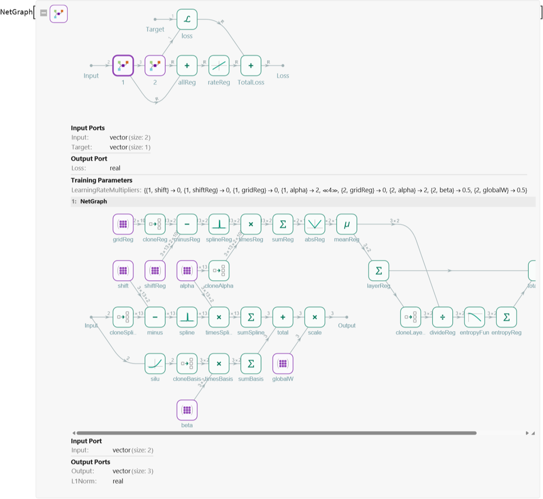
The NetGraph above shows the detailed architecture of the KAN:
1
.Upper Panel: Overall Workflow
1
.1
.Inputs: The network takes a vector input of size 2 (representing ,). A target output is provided for supervised learning (the true value ).
x
1
x
2
f(,)
x
1
x
2
1
.2
.Forward Pass: The main computational path is through one or more NetGraph layers—each is a KAN layer as introduced previously. The output of the last layer forms the network’s prediction, which is then compared to the target with a mean squared loss.
1
.3
.Regularization and Loss: In parallel to the main stream, each KAN layer computes regularization terms (L1 norm and entropy) to encourage sparsity and discreteness in learned functions.
The total loss used for optimization is a weighted sum of prediction error and regularization terms.
The total loss used for optimization is a weighted sum of prediction error and regularization terms.
2
.Lower Panel: A Single KAN Layer (Detailed View)
2
.1
.Spline Branch: The input is replicated and shifted by a grid of offsets, then passed through a B-spline basis layer. Learnable weights (alpha) combine the splines, and the result is summed to yield the nonlinear, univariate function for each edge.
2
.2
.SiLU/Residual Branch: In parallel, the input is passed through a SiLU (Swish) activation, then linearly weighted (beta) and added to the spline output. This “residual” pathway stabilizes training and helps capture any necessary linear structure.
2
.3
.Scaling and Aggregation: The outputs of both branches are summed, then globally scaled by another learnable parameter for each output node (globalW). The final output is thus a sum of learnable, flexible univariate functions.
2
.4
.Regularization Pipelines: In the upper part of the diagram, the network computes the L1 norm of each activation over a sample grid, and combines this with an entropy penalty measuring distributional discreteness.
Next, we train the KAN model over 100 rounds and obtain its loss.
Out[]=
| rounds |
loss |
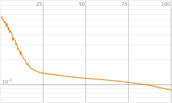
After training, we visualize the learned network structure. Edges and nodes are annotated to show importance and the learned shapes of the splines along each connection.
Out[]=
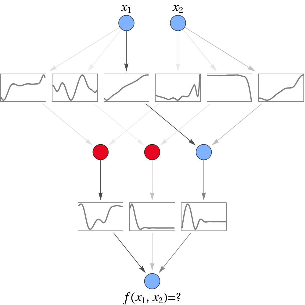
As we can see, the input variables and feed into a middle layer with three neurons, each receiving several potential nonlinear transformations (shown as inset plots of the learned splines) from the inputs. The colored nodes and edges indicate pathway activity: blue denotes active, high-contribution nodes, while red highlights less important ones, and greyed connections represent nearly zeroed (inactive) pathways. At this stage, the network has expressed the target function as a complex superposition of candidate univariate functions, some of which may be redundant or negligible.
x
1
x
2
Pruning the Network and Re-Training
Pruning the Network and Re-Training
Using the previous visualization, we identify and prune low-importance edges (colored red), retaining only informative connections for subsequent retraining.
Out[]=
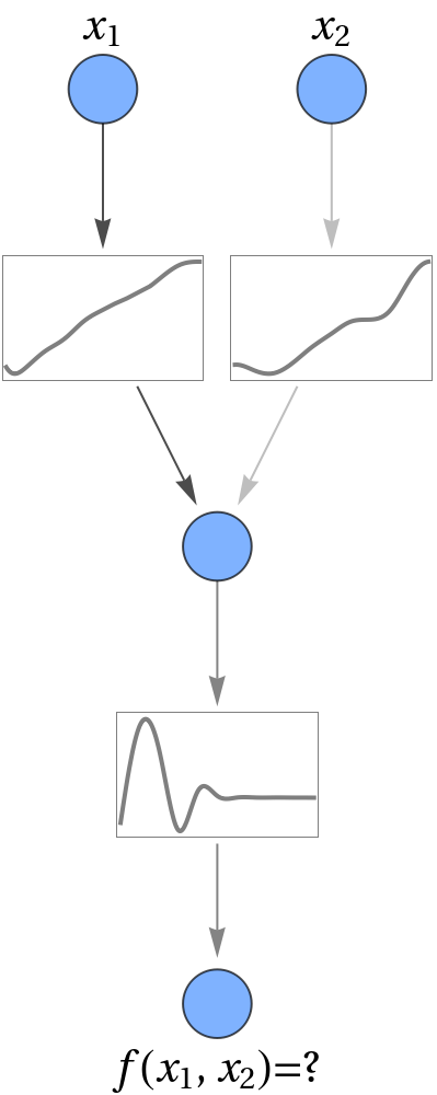
The architecture has now been greatly simplified, reducing to a single hidden node. This network is expected to efficiently re-learn the underlying functional relationship with far fewer parameters. To this end, we initialize and train a compact KAN to check if interpretability improvements come at the cost of significant fit quality loss.
We again visualize the structure and splines of the pruned KAN to confirm if the compact network has retained expressive capacity and interpretability.
Extracting an Interpretable Ansatz
Extracting an Interpretable Ansatz
Finally, inspired by the KAN’s decomposition, we use a symbolic ansatz to fit the data, testing if a human-interpretable closed-form can be found.
Data Generation and Visualization
Data Generation and Visualization
The above 3D plot visualizes the nontrivial structure of the function’s surface.
Training a Wide KAN
Training a Wide KAN
To capture the more complex function composition, we start with a wider network architecture than in Example 1, using five hidden neurons in the [2, 5, 1] structure.
The initial trained KAN architecture is a “rich” graph with many parallel nonlinear paths—necessary to represent the oscillatory and root components.
Pruning and Simplification
Pruning and Simplification
Redundant or low-importance paths are pruned, drastically simplifying the network to a single hidden neuron as [2, 1, 1], mirroring the minimal functional form.
The final visualized network directly shows that the KAN decomposed the input into two univariate transformations, then summed and exponentiated—closely aligning with the original function’s structure.
Formula Extraction and Validation
Formula Extraction and Validation
We propose a symbolic ansatz based on the target function:
Applying FindFit exactly recovers the parameters confirming that the pruned KAN has discovered and encoded the true analytic law inside its architecture.
Data Preparation and Target Function
Data Preparation and Target Function
Training a Wide KAN
Training a Wide KAN
To ensure flexibility for learning function composition, we again start with a somewhat wide KAN [2,5,1], with moderate regularization strength.
The initial trained KAN contains many nonlinear pathways across its hidden layer.
Pruning, Retraining, and Algebraic Discovery
Pruning, Retraining, and Algebraic Discovery
By pruning inactive or redundant pathways, the KAN can be simplified to a single hidden neuron as [2,1,1] architecture,
which is then retrained to convergence.
Unlike the first two examples, here the KAN demonstrates an ability to discover and represent a fundamental mathematical identity: the product of two numbers can equivalently be written as the exponential of the sum of their logarithms. This illustrates the power of KANs not just for function fitting, but for recovering hidden structure and offering alternative, interpretable formulae for familiar operations.
Concluding Remarks
Concluding Remarks
Summary
Summary
In this project, I implemented Kolmogorov–Arnold Networks (KANs) in the Wolfram Language to advance the discovery of interpretable symbolic relations in scientific data. Through a sequence of synthetic regression experiments, I demonstrated how KANs can efficiently learn, decompose, and reveal the hidden algebraic or functional structure behind multivariate datasets. The network’s architecture and visualization tools made the process transparent, showing explicitly how KANs reduce complex problems to understandable univariate transformations. Interestingly, KANs not only recovered target formulas but also uncovered mathematical identities, illustrating their potential for both accuracy and scientific insight.
Outlook
Outlook
The natural next stage is to apply KANs to real-world physical datasets, moving beyond synthetic data to tackle the challenges inherent in experimental science. This will require robust regularization, more advanced pruning techniques, and perhaps the integration of external symbolic regression or language model tools for extracting closed-form laws. Inspired by Stephen Wolfram’s vision [4] and the broader goals of the SymPhysAI project [5-7], my ambition is for KANs to become not just predictive engines but genuine collaborators in scientific discovery—helping researchers construct clear, interpretable narratives about the physical world. As we continue to refine these methods, I look forward to exploring their application to open problems in physics and related fields.
Acknowledgments
Acknowledgments
I thank Wolfram Summer School 2025 mentors, Nikolay Murzin and Jon Lederman, as well as Stephen Wolfram, Bowen Ping, Stephanie Bowyer, Xerxes Arsiwalla, and the Wolfram Summer School community for their guidance and support. I am also grateful to Mircea Trif for helpful discussions. I acknowledge the support from the European Union’s Horizon Europe research and innovation programme under the Marie Skłodowska-Curie Grant Agreement No. 101180589 (SymPhysAI). Views and opinions expressed are however those of the author(s) only and do not necessarily reflect those of the European Union or the European Research Executive Agency. Neither the European Union nor the granting authority can be held responsible for them.
References
References
1
.Z. Liu, Y. Wang, S. Vaidya, F. Ruehle, J. Halverson, M. Soljacic, T. Y. Hou, and M. Tegmark, KAN: Kolmogorov–Arnold Networks, in ICLR 2025 (2024).
2
.Z. Liu, P. Ma, Y. Wang, W. Matusik, and M. Tegmark, KAN 2.0: Kolmogorov-Arnold Networks Meet Science, arXiv:2408.10205 (2024).
3
.A. Hafver, Kolmogorov-Arnold networks (KANs) in Wolfram language, Wolfram Community, STAFF PICKS, (2024).
4
.5
.P.-X, Shen, Majorana-magnon interactions in topological Shiba chains, Wolfram Community, STAFF PICKS, (2024).
6
.P.-X, Shen, Non-Hermitian Fermi-Dirac distribution in persistent current transport, Wolfram Community, STAFF PICKS, (2024).
7
.Cite This Notebook
Cite This Notebook
Interpretable Symbolic Regression with Kolmogorov–Arnold Networks
by Peixin Shen
Wolfram Community, STAFF PICKS, July 9, 2025
https://community.wolfram.com/groups/-/m/t/3497558
by Peixin Shen
Wolfram Community, STAFF PICKS, July 9, 2025
https://community.wolfram.com/groups/-/m/t/3497558