CITE THIS NOTEBOOK: Axon-like circuits: self -assembled -controlled bioelectric networks growth by Russell Deaton. Wolfram Community DEC 1 2022.
ORIGINAL ARTICLE: Deaton, R., Garzon, M. & Yasmin, R. Systems of axon-like circuits for self-assembled and self-controlled growth of bioelectric networks. Scientific Reports, 12, 13371 (2022). https://doi.org/10.1038/s41598-022-17103-4.
ORIGINAL ARTICLE: Deaton, R., Garzon, M. & Yasmin, R. Systems of axon-like circuits for self-assembled and self-controlled growth of bioelectric networks. Scientific Reports, 12, 13371 (2022). https://doi.org/10.1038/s41598-022-17103-4.
Article Abstract: By guiding cell and chemical migration and coupling with genetic mechanisms, bioelectric networks of potentials influence biological pattern formation and are known to have profound effects on growth processes. An abstract model that is amenable to exact analysis has been proposed in the circuit tile assembly model (cTAM) to understand self-assembled and self-controlled growth as an emergent phenomenon that is capable of complex behaviors, like self-replication. In the cTAM, a voltage source represents a finite supply of energy that drives growth until it is unable to overcome randomizing factors in the environment, represented by a threshold. Here, the cTAM is extended to the axon or alternating cTAM model (acTAM) to include a circuit similar to signal propagation in axons, exhibiting time-varying electric signals and a dependence on frequency of the input voltage. The acTAM produces systems of circuits whose electrical properties are coupled to their length as growth proceeds through self-assembly. The exact response is derived for increasingly complex circuit systems as the assembly proceeds. The model exhibits complicated behaviors that elucidate the interactive role of energy, environment, and noise with electric signals in axon-like circuits during biological growth of complex patterns and function.
Introduction
Introduction
Over the course of several papers [1-4], we have investigated how electric signals and self-assembled growth interact to create complex biological structure and function. In the resulting circuit tile assembly models (cTAM), simple circuit tiles bind to a growing ladder assembly if the electric potential difference at the terminus is greater than a threshold. The voltage source () and the threshold ()represent a finite energy that is consumed as growth proceeds and randomizing forces in the environment, respectively. These simple, discrete models are amenable to exact analysis and have demonstrated remarkably complex behavior, such as self-controlled growth[1] and self-replication[2]. In this paper, the circuits are based upon those for propagation of action potentials in cable theory for axons, and the analysis is extended to the time and frequency domains. Thus, this axonal circuit tile assembly model (acTAM) shows how growth can produced complex signaling in axon-like networks. An example of an acTAM ladder circuit is shown in the figure below. Containing resistors and capacitors, the circuit tiles bind together through chemical glues (a-a’) as long as the electric potential difference at the tip exceeds the threshold. In this paper, assembly processes are monotonic, i.e., once a tile is attached, the attachment will never dissolve. [1] R. Deaton, M. Garzon, R. Yasmin, and T. Moore, "A model for self-assembling circuits with voltage-controlled growth," International Journal of Circuit Theory and Applications, vol. 48, no. 7, pp. 1017–031, 2020.[2] R. Yasmin, M. Garzon, and R. Deaton, "Model for self-replicating, self-assembling electric circuits with self-controlled growth," Phys. Rev. Research, vol. 2, p. 033165, Jul 2020.[3] Y. Yan, M. Garzon, and R. Deaton, "Harmonic circuit self-assembly in cTAM models," IEEE Transactions on Nanotechnology, vol. 18, pp. 195–99.[4] Y. Yan, M. Garzon, and R. Deaton, "Self-assembly of 2-d resistive electric grids," IEEE Transactions on Nanotechnology, vol. 18, pp. 562–66.
ν
0
τ
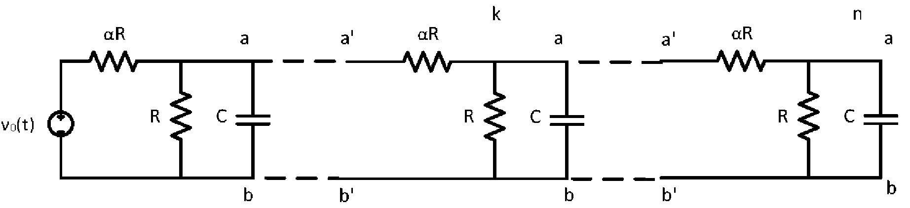
Complete Solution of the Axonal Circuit Tile Assembly Model
Complete Solution of the Axonal Circuit Tile Assembly Model
Nodal Analysis
Nodal Analysis
Kirchoff’s Current Law (KCL) is about conservation of charge and states that the sum of the currents entering and exiting any node in a circuit must be 0. Applying KCL, the equation for a node potential at a node k in the circuit is
ν
k
(2+α)--+αRC0.
ν
k
ν
k-1
ν
k+1
d
ν
k
dt
Under direct current (DC) or for phasor analysis, the system of differential equations can be written as ν, with the matrix of coefficients as
A
n
b
n
2+α | -1 | 0 | ⋯ | 0 |
-1 | ⋱ | ⋱ | ⋱ | ⋮ |
⋮ | -1 | 2+α | -1 | ⋮ |
⋮ | ⋱ | ⋱ | ⋱ | ⋮ |
0 | ⋯ | ⋯ | -1 | 1+α |
and the source vector as
ν 0 |
0 |
⋮ |
where (ω) is the source potential in the frequency domain.
ν
0
DC or Steady-State Solution
DC or Steady-State Solution
According to Cramer’s rule the node potentials are then ,where is the matrix with the k-th column of replaced with the source vector , and or a corresponding capital letter denotes the determinant of the corresponding matrix. Since is a tridiagonal matrix, the determinants satisfy a recurrence relation (2+α)- with 1+α and 0. The solutions to the characteristic equation for the recurrence are:
ν
k
(k)
A
n
A
n
(k)
A
n
A
n
(k)
A
n
A
n
b
n
·
A
n
A
n
A
k
A
k-1
A
k-2
A
1
A
0
In[]:=
Solve[ρ^k-(2+α)*ρ^(k-1)+ρ^(k-2)0,ρ]
Out[]=
ρ(2+α-(2+α+
1
2
α
4+α
),ρ1
2
α
4+α
)In[]:=
ρ1[α_]:=((2+α)+Sqrt[α*(α+4)])/2
In[]:=
ρ2[α_]:=((2+α)-Sqrt[α*(α+4)])/2
The general solution is, then, any linear combination +. With initial conditions 1+α and 1+3α+, the constants are
A
n
a
1
n
ρ
1
a
2
n
ρ
2
A
1
A
2
2
α
In[]:=
FullSimplify[Solve[{1+α*ρ1[α]+*ρ2[α],α^2+3*α+1==*ρ1[α]^2+*ρ2[α]^2},{,}]]
a
1
a
2
a
1
a
2
a
1
a
2
Out[]=
,-
a
1
4+α+
α(4+α)
8+2α
a
2
1
2
α
2
α(4+α)
In[]:=
a1[α_]:=1+
1
2
α
4+α
In[]:=
a2[α_]:=-
1
2
α
2
α(4+α)
Then, the expression for the determinant for a circuit with n nodes is
A
n
In[]:=
dk[α_,k_]:=a1[α]*ρ1[α]^k+a2[α]*ρ2[α]^k
The steady-state node potential at node k of n, (t), with a source potential offrom Cramer’s rule is:
ss
ν
k
ν
0
In[]:=
vs[α_,k_,n_,vo_]:=vo*dk[α,n-k]/dk[α,n]
This equation can be used not only for DC potentials but also for steady-state values of the node potentials with a complex α(1+jωRC) substituted for α.
′
α
In[]:=
ap[s_,α_,r_,c_]:=α+s*α*c*r
Using input parameters approximating those for an axon (ω, α, R, C,,T) (, and ),
ν
0
α, RΩ, CF
-6
10
12
10
-8
10
||100 mV
ν
0
In[]:=
pp={{0,10^(-6),10^(12),10^(-8),0.1,0.3}}
Out[]=
0,,1000000000000,,0.1,0.3
1
1000000
1
100000000
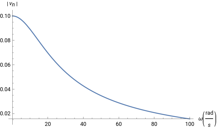
the magnitude of frequency response is
In[]:=
Plot[{ComplexExpand[Abs[vs[ap[*w,pp[[1,2]],pp[[1,3]],pp[[1,4]]],3,3,pp[[1,5]]]]]},{w,0,100},PlotRange->All,AxesLabel{HoldForm[ω[rad/s]],HoldForm[Abs[Subscript[ν,n]]]},PlotLabelNone,LabelStyle{GrayLevel[0]}]
Out[]=
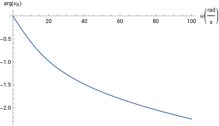
and the phase of the frequency response is
In[]:=
Plot[{ComplexExpand[Arg[vs[ap[*w,pp[[1,2]],pp[[1,3]],pp[[1,4]]],3,3,pp[[1,5]]]]]},{w,0,100},PlotRange->All,AxesLabel{HoldForm[ω[rad/s]],HoldForm[Arg[Subscript[ν,n]]]},PlotLabelNone,LabelStyle{GrayLevel[0]}]
Out[]=
Transient Response
Transient Response
As mentioned earlier, this solution is valid for DC and steady-state solutions. As the ladder grows, however, when a new circuit tile attaches to the ladder circuit, a transient response is generated. Thus, the acTAM actually represents a family of circuits, one for each length of the ladder, with their own electrical responses. For tridiagonal matrices, expressions for the eigenvalues and eigenvectors were found in the literature [5]. The transient response is given by (t)exp(t), where the eigenvalue is ,the value of the eigenvector is , and the areconstantsdeterminedfromtheinitialconditions.
{1,…,n}
tr
ν
k
n
∑
i0
b
i
χ
i,k
λ
i
th
i
λ
i
th
i
th
k
χ
i,k
b
i
Transient response: Eigenvalue k of n
In[]:=
ei[α_,r_,c_,k_,n_]:=(-(2+α)/(α*r*c)+(2/(α*r*c))*Cos[(2*k-1)*Pi/(2*n+1)])
Transient response: Eigenvectors j for eigenvalue k of n
In[]:=
ev[j_,k_,n_]:=Sin[(2*k-1)*j*Pi/(2*n+1)]
Transient response for node potential k of n eigenvalue and eigenvector j
In[]:=
vtr[α_,r_,c_,j_,k_,n_,t_]:=ev[j,k,n]*Exp[ei[α,r,c,k,n]*t]
[5] C . Fonseca and V . Kowalenko, "Eigenpairs of a family of tridiagonal matrices: three decades later," Acta Mathematica Hungarica, vol . 160.
Complete Solution
Complete Solution
Summary of the Analysis
Summary of the Analysis
For the analysis of the acTAM, the differential equations for a system of circuits are derived using nodal analysis (KCL). First, the system is solved for a non-time-varying (DC) case, which makes the capacitor an open-circuit and the circuit purely resistive . Then, using phasor analysis, the steady-state response in the frequency domain is derived from the DC equations with complex impedances. The expressions for the transient response were determined from results in the literature for tridiagonal matrices [5]. The arbitrary constants are then determined by the initial conditions, which are set by the values of the node potentials when a new ladder tile attaches.
[5] C . Fonseca and V . Kowalenko, “Eigenpairs of a family of tridiagonal matrices: three decades later,” Acta Mathematica Hungarica, vol . 160.
[5] C . Fonseca and V . Kowalenko, “Eigenpairs of a family of tridiagonal matrices: three decades later,” Acta Mathematica Hungarica, vol . 160.
Dynamics of Network Potentials from Growth
Dynamics of Network Potentials from Growth
Attachment of successive ladder tiles causes a propagation of the signals to the other tiles, which reconfigures the node potentials at the previous nodes into a new steady-state after a brief transient. The method of analysis is now demonstrated as a new tile attaches every T = 3 ms.
One Tile
One Tile
Two Tiles
Two Tiles
Solve for arbitrary constants using initial conditions for n = 2 (two tiles). The initial conditions for the first tile are the value of the node potential in the first tile (seed) at t = 3 ms when the second tile attaches. The initial condition for the second tile is 0 V since it is initially disconnected from the ladder and thus, the voltage source.
In[]:=
Node potential 1 of 2
Three Tiles
Three Tiles
The figure below shows the transient response as new tiles attached every 3 ms, before settling to new steady-state values.
Dependence on Reaction Conditions
Dependence on Reaction Conditions
Reaction Rate-Limited
Reaction Rate-Limited
One Tile
One Tile
Two Tiles
Two Tiles
Node potentials at k = 1 in ladder of length n = 2.
Node potentials at k = 2 in ladder of length n = 2.
Three Tiles
Three Tiles
Node potentials at k = 1,2, 3 in ladder of length n = 3.
Four Tiles
Four Tiles
The node potentials:
Diffusion-Limited
Diffusion-Limited
DC Input
DC Input
In an approximation to a diffusion-limited regime, tiles are available for binding at a fixed time interval T . Every T seconds, a new tile arrives at a growing ladder terminus and attaches if the terminal potential is at least τ . For the next example, a DC voltage source is applied at t = 0 and tiles arrive every T = 0.3 s .
One Tile
One Tile
Two Tiles
Two Tiles
Use initial conditions at multiples of the attachment period T = 0.3 s to determine arbitrary constants.
Node potentials at k = 1,2, in ladder of length n = 2.
Build the piecewise solution to show the steady-state value and the node potentials before and after attachment of the second tile.
Three Tiles
Three Tiles
Four Tiles
Four Tiles
In the figure below, there is relatively little attenuation as growth proceeds because the value of α is small compared to R for parameters approximating an axon. Once again, transients occur when new tiles attach.
Diffusion-Limited reaction with Sinusoidal Input
Diffusion-Limited reaction with Sinusoidal Input
Steady-State Sinusoidal Solution
Steady-State Sinusoidal Solution
One Tile
One Tile
Two Tiles
Two Tiles
Three Tiles
Three Tiles
Four Tiles
Four Tiles
Once again, attachment produces increasingly complex behavior, in which phase shifts and filtering characteristics are affected by growth.
Bounds on the Length of the acTAM Ladder
Bounds on the Length of the acTAM Ladder
Bounds on the growth of the acTAM circuit as frequency of the input varies. Growth is attenuated at higher frequences, and thus, acts like a low-pass filter, just like axons.
Conclusions
Conclusions
Living systems transduce flows of energy and matter from the environment to grow, produce complex biological patterns, respond to sensory input, and reproduce. Because of their complexity, it is a challenge to model the input-output relationships among the various flows into the system and predict the response, be that a structure or a behavior. The acTAM enables self-controlled growth driven by a finite source of energy (voltage source) in a background environment (threshold). This complex and characteristic behavior comes as a direct consequence of the interaction among components of the model that are proxies for components in a biological network, namely matter (represented by circuit tiles), energy (input voltages), communication (through signal propagation and dynamic interaction among components representing somatic computation without a central information processor) and interaction with the environment (dynamic growth to homeostasis) at various levels of abstraction. The acTAM circuit is highly similar to that of axonal cable theory, which at this stage, is its most appropriate benchmark. The acTAM is a tool that enables exploration of the interaction between electric potentials that depend on the growth of a biological structure, and vice versa. Growth itself introduces more complicated time-varying behavior, and additional frequency components in the signal. Transduction of energy to overcome disorder through growth of organized structures would seem to be a prerequisite for early life, and at least in its electric signals, the acTAM starts to demonstrate how those early growth mechanisms may have contributed to the development of complex biological shape and function.
In conclusion, the acTAM offers the potential to uncover deep clues on the etiology of biological structure formation (shape and dynamics). For example, what really controls and limits growth is access to environmental resources and the coupling
between components and the environment. It also captures mechanisms that couple growth and electrical signaling in axon-like networks with predictive capability for both length and electrical response. These models also provide full and realistic examples of the well known property of autopoiesis, in which the structure of an organism is determined and preserved by, not in spite of, interaction between components and the environment. Furthermore, the model itself (although not the analysis) is relatively simple and so affords the possibility of models for more complex and realistic phenomena (proteins and neuronal assemblies) in which the representation of matter is less abstract than in conventional models and closer to direct electrical phenomena. These properties would also allow the possibility of providing a more objective and systematic framework to address issues such as homeostasis, self-healing, and other epigenetic biological phenomena as emergent properties rather than being explicitly programmed.