ABSTRACT (original article): We analyze truncated series generated as divergent formal solutions of non-linear ordinary differential equations. Motivating the study is a specific non-linear, first-order differential equation, which is the basis of the resurgent formulation of renormalized perturbation theory in quantum field theory. We use the Borel–Padé approximant and classical analysis to determine the analytic structure of the solution using the first few terms of its asymptotic series. Afterward, we build an approximant, consistent with the resurgent properties of the equation. The procedure gives an approximate expression for the Borel–Ecalle resummation of the solution useful for practical applications. Connections with other physical applications are also discussed. CITATION (original article): Maiezza, A.; Vasquez, J.C. Uncovering Hidden Patterns: Approximate Resurgent Resummation from Truncated Series. Mathematics 2024, 12, 3087. https://doi.org/10.3390/math12193087
This notebook demonstrates the calculation of resurgent approximations for non-perturbative results in quantum field theory (QFT) perturbation series.
Section 1 begins with simple examples using Padé analysis to approximate well-known series. Section 2 explores the application of the Padé approach to specific examples within the framework of ordinary differential equations (ODEs), demonstrating its limitations in capturing complete solutions.
Section 3 presents a classical analysis using Padé approximation to determine the analytic structure of solutions for both linear and non-linear ODEs, working with truncated series solutions. This analysis is motivated by the truncated series encountered in perturbative QFT calculations. The section shows how classical analysis can reveal both the location of the singularities in the Borel transform of the solution, as well as the analytic structure from their truncated series.
Section 3 presents a classical analysis using Padé approximation to determine the analytic structure of solutions for both linear and non-linear ODEs, working with truncated series solutions. This analysis is motivated by the truncated series encountered in perturbative QFT calculations. The section shows how classical analysis can reveal both the location of the singularities in the Borel transform of the solution, as well as the analytic structure from their truncated series.
Sections 4 and 5 introduce the main novel analysis, presenting a suitable approximants for ODE solutions using modern resurgence techniques developed by Ecalle and Costin. We provide an algorithmic implementation in Wolfram Mathematica for Alien calculus techniques with their associated resurgence and medianization operations for ODEs in their “normal form.” This new procedure is shown to outperform classical analysis and capture non-perturbative information that standard procedures miss.
Finally, sections 6 and 7 explore additional examples with more general analytic structures for the Borel transform of the solution. These sections compare the resurgence approach with an alternative approximation scheme using Meijer-G functions, demonstrating the superior performance of resurgence-based approximation techniques.
Main Calculation
Main Calculation
1- Padè examples
1- Padè examples
Start from a an exponential
"Example of Padè"PadeApproximant[,{x,0,3}]Series[%,{x,0,8}]Series[,{x,0,8}]
x
x
Example of Padè
3
x
120
2
x
10
x
2
-+-+1
3
x
120
2
x
10
x
2
1+x++++++++O()
2
x
2
3
x
6
4
x
24
5
x
120
6
x
720
7
x
4800
8
x
28800
9
x
1+x++++++++O()
2
x
2
3
x
6
4
x
24
5
x
120
6
x
720
7
x
5040
8
x
40320
9
x
x
x
x
54.5982
77.
54.2444
53.4317
pd=PadeApproximant[,{x,0,3}];ss=Series[,{x,0,6}]//Normal;LogPlot+ss,+pd,{x,0,4},PlotStyle{Yellow,Red}
x
x
Abs[ss-]
x
x
Abs[pd-]
x
x
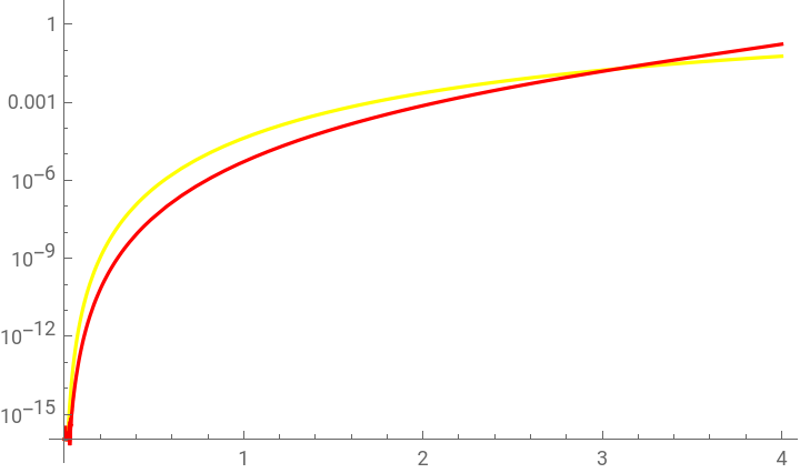
Divergence of the approximant
Solve[Denominator[pd]0,x,Reals]//Flatten//N
{x4.64437}
Reproduce now some result of the reference below.
http://www.scholarpedia.org/article/Pad%C3%A9_approximant
http://www.scholarpedia.org/article/Pad%C3%A9_approximant
Clear[f]f[x_]:=DLog×+,xn=.;tt=Tablepd=PadeApproximant[f[x],{x,0,n}];solx=Solve0,<x<,x,Reals//Flatten;{solx//N,Table[Residue[pd,{x,(x/.solx〚i〛)}]//N,{i,1,CountDistinct[solx]}]},{n,2,9}
-3/2
(1-x)
3/2
1-x
1
2
-x
1
pd
9
10
11
10
{x0.966036} | {-1.25063} |
{x0.965263} | {-1.2477} |
{x1.00471} | {-1.60153} |
{x1.0017} | {-1.54827} |
{x1.00034} | {-1.51563} |
{x1.00035} | {-1.51605} |
{x1.00009} | {-1.50651} |
{x1.00005} | {-1.50443} |
2 - Samples of normal nonlinear ODE: exact vs series approximation
2 - Samples of normal nonlinear ODE: exact vs series approximation
Nonlinear ODE with simple poles (in 1,2,3...)
Nonlinear ODE with simple poles (in 1,2,3...)
Series approximated solution
NN=30;eq=y'[x]--y[x]++/.yFunctionx,a[n]//Expand/.0/;aa≤-(NN+1)//ExpandAll;Table[=Coefficient[eq,x,(1-i)]0,{i,1,NN+1}];Clear[sol]sol=Solve[,a[0]]〚1〛//Flatten;listsol=Table[sol=(Append[sol,(Solve[/.sol,a[i-1]])〚1〛])//Flatten,{i,2,NN+1}]//Flatten//DeleteDuplicates;listcol=%//Column
1
x
2
y[x]
NN
∑
n=0
-n
x
aa_
x
cc
i
cc
1
cc
i
a(0)0 |
a(1)1 |
a(2)2 |
a(3)8 |
a(4)44 |
a(5)296 |
a(6)2312 |
a(7)20384 |
a(8)199376 |
a(9)2138336 |
a(10)24936416 |
a(11)314142848 |
a(12)4252773824 |
a(13)61594847360 |
a(14)950757812864 |
a(15)15586971531776 |
a(16)270569513970944 |
a(17)4959071121374720 |
a(18)95721139472072192 |
a(19)1941212789888952320 |
a(20)41271304403571227648 |
a(21)918030912312297752576 |
a(22)21325054720042613565440 |
a(23)516411258045443243712512 |
a(24)13015974776063736935370752 |
a(25)340945321133652566502662144 |
a(26)9268634751928324124569690112 |
a(27)261159656529092893640320385024 |
a(28)7617784632051754134442268278784 |
a(29)229768246328872907611261136568320 |
a(30)7158581937628933666777995949015040 |
"Show that, for large enough n, the a(n) go like n! (n-3):"Table[{n!(n-3)(*approximatebehaviorforlargen--tocheck*),a[n]/.listsol},{n,4,20}]
Show that, for large enough n, the a(n) go like n! (n-3):
24 | 44 |
240 | 296 |
2160 | 2312 |
20160 | 20384 |
201600 | 199376 |
2177280 | 2138336 |
25401600 | 24936416 |
319334400 | 314142848 |
4311014400 | 4252773824 |
62270208000 | 61594847360 |
958961203200 | 950757812864 |
15692092416000 | 15586971531776 |
271996268544000 | 270569513970944 |
4979623993344000 | 4959071121374720 |
96035605585920000 | 95721139472072192 |
1946321606541312000 | 1941212789888952320 |
41359334139002880000 | 41271304403571227648 |
Let us compare the approximated series solution with the exact one.
Nonlinear ODE with branch points (in 1,2,3...)
Nonlinear ODE with branch points (in 1,2,3...)
Series approximated solution
Compare exact solution and the series approximation
3 - Padè to study the ODE analytic structure from a truncated series
3 - Padè to study the ODE analytic structure from a truncated series
Linear ODE (Euler equation)
Linear ODE (Euler equation)
Finally, check the case of a single pole, from Euler equation
Nonlinear ODE with simple poles
Nonlinear ODE with simple poles
Checking the poles of Borel-Padè
For comparison, now do the same on LerchPhi:
Linear ODE but with one branch point
Linear ODE but with one branch point
An important trick is to take the padè of derivative - of - Log (see also the Section “Padè examples”). The reason is to trasnform the initial input series (pointing to a branch point) into a series pointing to a pole
Try to Distinguish the kind of branch points in nonlinear ODEs
Try to Distinguish the kind of branch points in nonlinear ODEs
The idea of this section relies on the trick of derivative-of-log that, in principle, allows to capture the kind of root-branch-points -- it is given by “b” in this example
WE IMPLEMENT THIS IDEA ON THE BOREL-PADE’ APPROXIMANT, FOCUSING ON THE CLOSEST SINGULARITY TO 1 (WHICH IS THE FIRST SINGULARITY IN BOREL SPACE)
4 - Approximant for ODE with simple poles
4 - Approximant for ODE with simple poles
Approximant convergence
Approximant convergence
The proposed approximant
Convergence of the above approximant
Approximant convergence 2 -- more denominators
Approximant convergence 2 -- more denominators
The proposed approximant
Convergence of the above approximant
New attempt: N’ as a function of N
Build the approximant : the formal one is PD; the actual one in exBPD
Showing the Final result
5 - Approximant for ODE with branch points
5 - Approximant for ODE with branch points
Build the approximant : the formal one is PD; the actual one in exBPD
Given the above approximant of the Borel transform exBPD, we do the Principal Value of the Laplace transform. We can only do numerically (here, integrating up to z=20 approximates very well ∞). This step enable us to approximate the PV:
Final result with higher nonperturbative sectors
Final result with higher nonperturbative sectors
Showing the Final result
7 - Meijer-G approximation (to compare for simple poles)
7 - Meijer-G approximation (to compare for simple poles)
Meijer-G approximation, at leading order (no solution)
Meijer-G approximation, at higher order:
By contrudction, the Borel transform of M is (eq.8 of Mera):
Other examples
Other examples
CITE THIS NOTEBOOK
CITE THIS NOTEBOOK
Uncovering hidden patterns: approximate resurgent resummation from truncated series
by Alessio Maiezza & Juan Carlos Vasquez
Wolfram Community, STAFF PICKS, October 31, 2024
https://community.wolfram.com/groups/-/m/t/3312448
by Alessio Maiezza & Juan Carlos Vasquez
Wolfram Community, STAFF PICKS, October 31, 2024
https://community.wolfram.com/groups/-/m/t/3312448