ABSTRACT (original article): Understanding the solvation structure of the hydrated electron, an excess electron in bulk water, has been a long-standing challenge. Experiments have shown that the solvation entropy, which encodes how the water molecules near the electron behave, is anomalously large and positive for the hydrated electron. Here, we use semiclassical and ab initio alchemical simulations to calculate the solvation entropy of several simulation models of the hydrated electron, including ab initio density functional theory (DFT) with a hybrid GGA functional. We find that cavity-forming one-electron models with relatively soft cavities correctly predict the sign of the hydrated electron’s solvation entropy but underestimate its magnitude. Both a noncavity one-electron model and hard cavity-forming DFT yield an incorrect sign for the solvation entropy. The calculated solvation entropies of each model are consistent with the structure and dynamic behavior of the first-shell waters molecules. CITATION (original article): William R. Borrelli, Xiaoyan Liu, and Benjamin J. Schwartz, The Solvation Entropy of Different Simulation Models of the Hydrated Electron, J. Phys. Chem. Lett. 2026, 17, 7, 1899–1906. https://doi.org/10.1021/acs.jpclett.5c02808
Introduction
Introduction
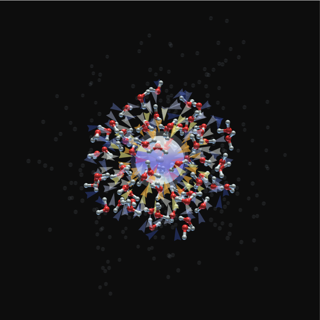
This notebook describes how we used our hydrated electron simulation data and Wolfram Mathematica to create our journal cover art for The Journal of Physical Chemistry Letters: https://pubs.acs.org/toc/jpclcd/17/7
Helper Functions
Helper Functions
Create Cover Art
Create Cover Art
First, load in XYZ coordinates from a molecular dynamics snapshot. This simulation contains water molecules and the final entry is the hydrated electron center of mass.
pos=ReadList["<<<your_file_path>>","String"];pos=ToExpression[StringSplit/@pos[[3;;]]];
Pull out waters in the first and second solvation shells of the hydrated electron.
fsWats=Select[Thread[{mmcNoPbc[pos[[-1]][[2;;]],Partition[pos[[1;;-2]][[All,2;;]],3][[All,1]],15.66],Partition[pos[[1;;-2]][[All,2;;]],3]}],#[[1]]<=3.3&][[All,2]];ssWats=Select[Thread[{mmcNoPbc[pos[[-1]][[2;;]],Partition[pos[[1;;-2]][[All,2;;]],3][[All,1]],15.66],Partition[pos[[1;;-2]][[All,2;;]],3]}],(#[[1]]>3.3)&&(#[[1]]<5.)&][[All,2]];
Create the vectors that highlight water-electron solvation. Closer vectors are longer and have warmer colors, while farther vectors are shorter and have cooler colors.
vectorFieldGraphics=Graphics3D[Table[Module[{vec=vector[x,y,z],r=Norm[{x,y,z}],alpha,strength,color,scaledVec},strength=1-Clip[(r-2.5)/5,{0,1}];scaledVec=0.5*strength*vec;alpha=0.8Exp[-0.02r^2];color=ColorData["TemperatureMap"][strength];{Opacity[alpha],color,Arrow[{{x,y,z},{x,y,z}+scaledVec}]}],{x,-5,5,2},{y,-5,5,2},{z,-5,5,2}],Boxed->False];
Make a glowing spherical hydrated electron with a halo effect.
sphereGraphics=Graphics3D[{Glow[Blue],Specularity[White,30],Opacity[0.5],Sphere[{0,0,0},2.5],Opacity[0.1],Glow[Blue],Sphere[{0,0,0},3.0]}];
Define options for how water molecules will be plotted.
molOpts=;
Plot first and second shell water molecules.
fsMol=MoleculePlot3D[makeMol[Map[#-pos[[-1]][[2;;]]&/@#&,fsWats]],Evaluate[Sequence@@molOpts]];ssMol=MoleculePlot3D[makeMol[Map[#-pos[[-1]][[2;;]]&/@#&,ssWats]],Evaluate[Sequence@@molOpts]];
Sample and plot “bulk” particles as semi-transparent spheres in the background.
nBulk=300;bulkMolecules=(SeedRandom[2024];Graphics3D[Table[{Opacity[0.05],LightBlue,Sphere[RandomReal[{-10,10},3],0.2]},{i,1,nBulk}]]);
Combine graphics to produce the cover.
ShowvectorFieldGraphics,sphereGraphics,fsMol,ssMol,bulkMolecules,
Output is the graphic:
CITE THIS NOTEBOOK
CITE THIS NOTEBOOK
The solvation entropy of different simulation models of the hydrated electron
by Will Borrelli
Wolfram Community, STAFF PICKS, February 25, 2026
https://community.wolfram.com/groups/-/m/t/3645288
by Will Borrelli
Wolfram Community, STAFF PICKS, February 25, 2026
https://community.wolfram.com/groups/-/m/t/3645288