This project seeks to further explore spacetime discretization through Wolfram-based hypergraph transformation dynamics, in which causal sets are effectively generated algorithmically via an abstract rewriting system defined over hypergraphs—an approach to causal set theory previously outlined by J. Gorard—while motivated by the causal dynamical triangulation (CDT) formalism and the associated procedures of R. Loll and B. Ruijl's locally causal dynamical triangulations (LCDT) . This article specifically seeks to examine a BoundaryMesh-based framework for loose corresponding interpretations of Euclidean and Lorentzian space, and apply these visualizations and operators to more grounded interpretations of some of the mathematical concepts featured in CDT and LCDT.
Introduction
Introduction

The construction of a unified model that explains the phenomena of both quantum mechanics and general relativity—the famed issue of quantum gravity—remains one of the most significant problems of physics and science as a whole. The most well-developed and well-known proposal is that of bosonic string theory, but string theory is a framework considered fundamentally flawed by some due to its focus on grand, somewhat arbitrary physical assumptions about the structure of the universe that better lend itself to mathematicians than scientists looking for a physical theory. Causal set theory, however, responds to this lack of physicality through its emphasis on a more general type of phenomenon familiar to every inhabitant of the Universe: that of cause and effect, which has mathematical significance at all length scales. More formally, causal set theory explores the invariance of the causal structure of Lorentzian manifold under conformal transformations, changes of coordinates →(σ) that scale the metric by some function of space squared such that (σ)→(σ)(σ); this allows causal set theory to concern itself with continuous spacetimes arbitrarily well-approximated by finite set of events, known as causal sets, with causal partial order relations upon them. Causal dynamical triangulation (CDT) is closely related: both CDT and causal sets attempt to model spacetime with a discrete causal structure, but while the causal set approach is relatively general, CDT assumes a more specific relationship between the lattice of spacetime events and geometry with a Lagrangian constrained by enough initial conditions as to be numerically analyzed—causal sets are far more topologically generic.This article explores a fairly straightforward version of CDT, the 1+1 case (one spatial dimension, one temporal dimension with a (+,-) metric signature), with conditions that are fairly easy to demonstrate with Wolfram's graph manipulation and generation functions. In particular, the majority of the investigation will be spent on comparing and contrasting different mathematical, physical, and visualizable properties of graphs with arbitrarily-assigned and coordinatized causal relationships: networks with arbitrarily assigned causal relationships that correspond loosely to a Lorentzian case, and coordinatized networks in Euclidean space with calculable Minkowski norms, respectively. This may give more concrete insight into the circumstances that define causal dynamical triangulation and the topological specificity that distinguishes it from the more generic causal set theory.
μ
σ
μ
σ
g
μν
2
Ω
g
μν
Arbitrary Triangulation
Arbitrary Triangulation
We will begin with a procedure that constructs triangulation by arbitrarily classifying edges as spacelike or timelike: in this way, we are forming a non-coordinatized system based on the predetermined assignment of causal relationships as opposed to any norm-based calculations.
As previously described, CDT is based upon various types of simplices, generalized triangles such that a 1-simplex is a line segment, a 2-simplex is a triangle, a 3-simplex is a tetrahedron, et cetera. We begin with BoundaryMeshRegion[{p1,...,pn}, Line{...}] which yields a mesh defined by a boundary with coordinates p1,...,pn, as outlined by Line{...}. We can then triangulate this result—in CDT parlance, divide graph into 1-simplices—and use Graph[] and MeshConnectivityGraph[...] to obtain a triangulated graph.
We begin with a simple type region, .
As previously described, CDT is based upon various types of simplices, generalized triangles such that a 1-simplex is a line segment, a 2-simplex is a triangle, a 3-simplex is a tetrahedron, et cetera. We begin with BoundaryMeshRegion[{p1,...,pn}, Line{...}] which yields a mesh defined by a boundary with coordinates p1,...,pn, as outlined by Line{...}. We can then triangulate this result—in CDT parlance, divide graph into 1-simplices—and use Graph[] and MeshConnectivityGraph[...] to obtain a triangulated graph.
We begin with a simple
BoundaryMesh[...]
ℛ
In[]:=
ℛ=BoundaryMeshRegion[{{0,0},{1,0},{1,1},{0,1}},Line[{1,2,3,4,1}]]
Out[]=

To convert this into the type of discretized region, we may define the following helper functions: GetTriangulatedPlaneEdgeList and GetTriangulatedPlaneGraph.
In[]:=
GetTriangulatedPlaneEdgeList[triangulatedGraph_]:=DirectedEdge@@#&/@EdgeList[triangulatedGraph];GetTriangulatedPlaneGraph[region_]:=MeshConnectivityGraph[TriangulateMesh[region]];GenerateTriangulatedMeshAdjaceny[region_]:=Module[ {triangulatedPlaneGraph,triangulatedPlaneVertexList, triangulatedPlaneEdgeList}, triangulatedPlaneGraph = GetTriangulatedPlaneGraph[region]; triangulatedPlaneEdgeList=GetTriangulatedPlaneEdgeList[triangulatedPlaneGraph]; triangulatedPlaneVertexList=VertexList[triangulatedPlaneGraph]; Graph[triangulatedPlaneEdgeList,VertexLabels->Placed["Name",Tooltip]]]triangulatedGraph = GetTriangulatedPlaneGraph[ℛ];triangulatedPlaneEdgeList = GetTriangulatedPlaneEdgeList[GetTriangulatedPlaneGraph[ℛ]];triangulatedPlaneVertexList=VertexList[GetTriangulatedPlaneGraph[ℛ]];
Column[{triangulatedGraph,GenerateTriangulatedMeshAdjaceny[ℛ]}]
Out[]=
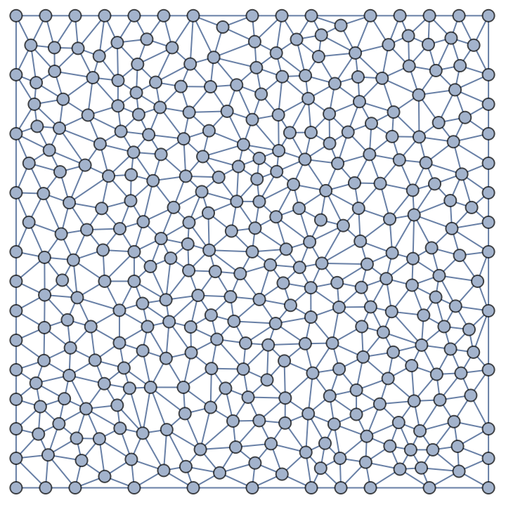
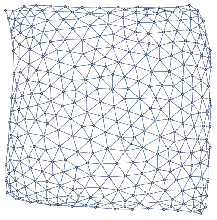
We can now create a function, , that takes the edge list of the triangulated region and creates a randomly generated association corresponding approximately half of the edges with a timelike value ("T") and the other half with a spacelike value ("S").
randomTimelikeAssigner
In[]:=
randomTimeLikeAssigner[triPlaneEdgeList_]:=Association[With[ {randomSubset=RandomSample[triPlaneEdgeList,Floor[Length[triPlaneEdgeList]/2]]}, If[ MemberQ[randomSubset,#], #->"T", #->"S" ]&/@triPlaneEdgeList]]updateGraphEdgeAssoc[vertex_]:=Association[ If[ MatchQ[Head[#], UndirectedEdge], #->"S", #->"T" ]&/@vertex];
The resulting association informs most of the visualization employed for the triangulated BoundaryMesh and how causal relationships between different nodes of the network are defined. One part of the former is undirecting edges assigned spacelike, implemented with UndirectIfSpacelike—as well as, for the sake of completion, UndirectIfSpacelikeOrLightlike.
We now approach the issue of causality in CDT: specifically, that locally causal dynamical triangulations should exhibit well-behaved vertices strictly surrounded by four timelike edges. This can be achieved fairly straightforwardly via IncidenceList:
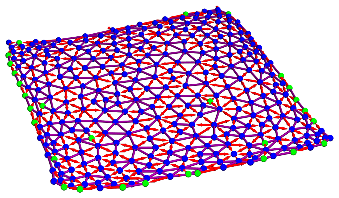
We should now be able to graph 3-dimensional graphs that present this locally-causally acceptable behavior through a visualization that incorporates three key pieces of causal information: (1) whether connections are spacelike, lightlike, or timelike, denoted through colors set in the original arbitrarily-assigned association; (2) preserved arbitrarily defined causal directions defined through the original convention with the all-directed BoundaryMesh; and (3) whether vertices are causally appropriate or not in Loll's 1+1 CDT local causality condition, for which points are green if the rule is violated and blue if they are appropriate.
We proceed to define the following Module for
As can be seen in the final graph, there are a number of events that violate this condition of local causality, thereby only making the network valid should these points be removed as to still form a triangulated surface consisting of these elemental (1,1) Minkowski triangles in accordance to local gluing rules; basic functions for such approaches are below.
Coordinatized Triangulation
Coordinatized Triangulation
With this procedure, we can examine the graph as it grows increasingly refined through repeatedly applying pruneIncidenceLists[].
Analysis and Physical Assessment
Analysis and Physical Assessment
Conclusion
Conclusion
This article demonstrated that the built-in triangulation features in the Wolfram language can allow for a basic framework of CDT, most assisted by the theory's conditions and gluing rules that ultimately distinguish it from causal set theory. In particular, Mathematica's visualizations enabled a clear comparison of causal network representations of simplicial triangulation decompositions in a non-coordinatized, loose version of Lorentzian space and connectivity graphs in undirected Euclidean space allowing for a straightforward inspection of otherwise more topologically generic concepts, like the various dimensional estimators discussed in this article.
Areas for Further Exploration
Areas for Further Exploration
Given that this project serves as a basic overview of the conditions enforced by CDT in Wolfram and the transition of past models of causal set theory in Mathematica to more strictly-defined frameworks of causal dynamical triangulation, the areas of the present article that can be further explored is directly tied to current issues in computational CDT (and quantum gravity as a whole). One particular topic of interest would be to better explore these conditions in the continuum limit, for which this model should exhibit attributes of Hořava–Lifshitz gravity (most notably, Petr Hořava's assertion that space and time are anisotropic at high energy levels) that correspond to mathematical behaviors observable in Wolfram-based models of quantum gravity. Another interesting project would be to more deeply explore the computational aspects of partition function calculation with this framework, which would likely require employing Metropolis-Hastings-like Monte Carlo algorithms for incrementally assessing differences between one triangulated configuration and another in CDT space.
Acknowledgements
Acknowledgements
I would like to gratefully acknowledge Megan Davis for helping organize my certifiably messy code and intervening with my lambda calculus addiction, as well as Jonathan Gorard for proposing a large part of this project and being so willing to let a Wolfram High School Summer Camp student further explore his original research.
Keywords
Keywords
◼
Causal dynamical triangulation
◼
Causal set theory
◼
Triangulation
◼
Causality