This notebook shows the calculation of gluon self-energy in massless Quantum Chromodynamics using FeynCalc 10 https://feyncalc.gitub.io and FeynArts https://www.feynarts.de. CITATION: Vladyslav Shtabovenko (2023), FeynCalc goes multiloop, J. Phys.: Conf. Ser. 2438 012140. https://doi.org/10.1088/1742-6596/2438/1/012140
Load FeynCalc and FeynArts
Load FeynCalc and FeynArts
In[]:=
$LoadAddOns={"FeynArts"};<<FeynCalc`$FAVerbose=0;
FeynCalc 10.0.0 (dev version, 2024-05-17 15:43:22 +02:00, ad9fc8fe). For help, use the onlinedocumentation, visit the forum and have a look at the supplied The PDF-version of the manual can be downloaded here.
If you use FeynCalc in your research, please evaluate FeynCalcHowToCite[] to learn how to cite this software.
Please keep in mind that the proper academic attribution of our work is crucial to ensure the future development of this package!
FeynArts 3.11 (3 Aug 2020) patched for use with FeynCalc, for documentation see the or visit www.feynarts.de.
If you use FeynArts in your research, please cite
• T. Hahn, Comput. Phys. Commun., 140, 418-431, 2001, arXiv:hep-ph/0012260
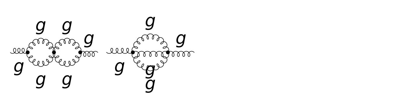
Generate Feynman diagrams using FeynArts
Generate Feynman diagrams using FeynArts
In[]:=
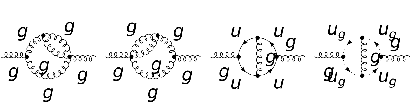
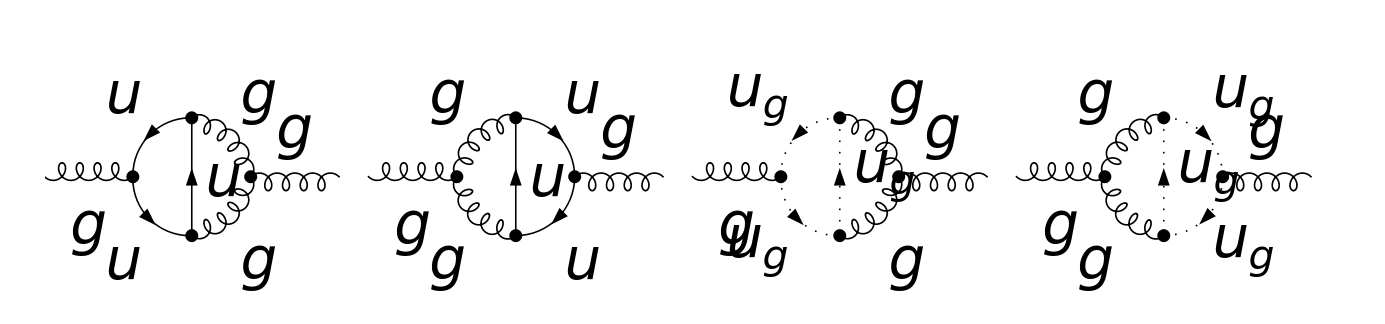
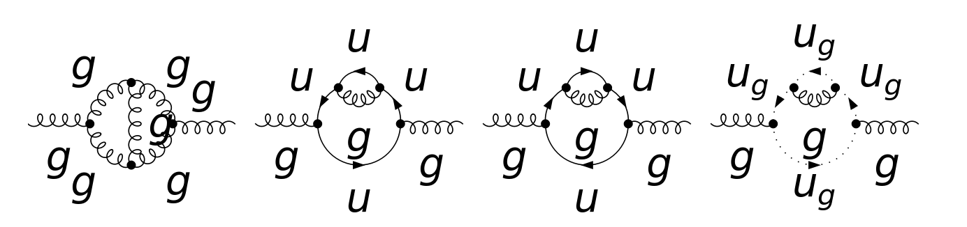
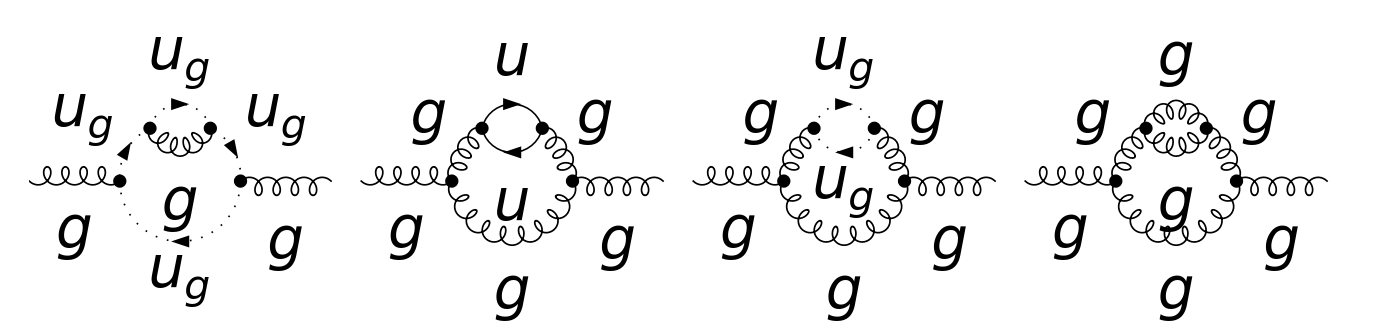
diags=InsertFields[CreateTopologies[2,1->1,ExcludeTopologies->{Tadpoles}],{V[5]}->{V[5]},InsertionLevel->{Particles},ExcludeParticles->{V[1|2|3],S[_],F[1|4],F[3,{2|3}]},Model->SMQCD];
In[]:=
Paint[DiagramExtract[diags,{2,3,4,5,6,7,8,9,10,11,12,13,14,15,16,17,20,39}],ColumnsXRows->{4,1},SheetHeader->False,Numbering->True,ImageSize->{1024,256}];
Convert the FeynArts output into valid FeynCalc input
Convert the FeynArts output into valid FeynCalc input
In[]:=
ampRaw=FCFAConvertCreateFeynAmpDiagramExtract[diags,{2,3,4,5,6,7,8,9,10,11,12,13,14,15,16,17,20,39}],Truncated->True, PreFactor->1,IncomingMomenta->{p},OutgoingMomenta->{p},LoopMomenta->{q1,q2}, UndoChiralSplittings->True,ChangeDimension->D,List->True,SMP->True, DropSumOver->True//SMPToSymbol;
Fix the kinematics
Fix the kinematics
In[]:=
FCClearScalarProducts[];ScalarProduct[p,p]=pp;
Calculation of the amplitude
Calculation of the amplitude
Define a projector that extracts Π(p^2) from +)Π(p^2)
(-
μν
g
μ
p
ν
p
2
p
In[]:=
projector=MTD[Lor1,Lor2]1/((D-1)SPD[p])1/(2CACF)SUNDelta[Glu1,Glu2]
Out[]=
Lor1Lor2
g
Glu1Glu2
δ
2(D-1)
2
p
C
A
C
F
Set the quark mass to zero and simplify the Dirac and color algebras
In[]:=
AbsoluteTiming[ampSimp=(projectorampRaw/.mu->0)//Contract//DiracSimplify//SUNSimplify;]
In[]:=
ampSimp
Identify and minimize the topologies
Identify and minimize the topologies
Identify the occurring topologies.
In[]:=
{amp,topos}=FCLoopFindTopologies[ampSimp,{q1,q2}];
FCLoopFindTopologies: Number of the initial candidate topologies: 6
FCLoopFindTopologies: Number of the identified unique topologies: 5
FCLoopFindTopologies: Number of the preferred topologies among the unique topologies: 0
FCLoopFindTopologies: Number of the identified subtopologies: 1
Integral topologies present in the amplitude
In[]:=
topos
Out[]=
FCTopologyfctopology1,,,,,,{q1,q2},{p},{Hold[Pair][p,p]pp},{},FCTopologyfctopology2,,,,,{q1,q2},{p},{Hold[Pair][p,p]pp},{},FCTopologyfctopology3,,,,,{q1,q2},{p},{Hold[Pair][p,p]pp},{},FCTopologyfctopology4,,,,,{q1,q2},{p},{Hold[Pair][p,p]pp},{},FCTopologyfctopology5,,,,{q1,q2},{p},{Hold[Pair][p,p]pp},{}
1
(+η)
2
q2
1
(+η)
2
q1
1
(+η)
2
(q1+q2)
1
(+η)
2
(p+q1)
1
(+η)
2
(p-q2)
1
(+η)
2
q2
1
(+η)
2
q1
1
(+η)
2
(q1+q2)
1
(+η)
2
(p-q1)
1
(+η)
2
q2
1
(+η)
2
q1
1
(+η)
2
(p+q2)
1
(+η)
2
(p-q1)
1
(+η)
2
q2
1
(+η)
2
q1
1
(+η)
2
(p-q1)
1
(+η)
2
(p-q1+q2)
1
(+η)
2
q2
1
(+η)
2
q1
1
(+η)
2
(p+q1+q2)
Final all nonvanishing subtopologies
In[]:=
subtopos=FCLoopFindSubtopologies[topos];
Uncover mapping relations between smaller and larger topologies
In[]:=
mappings=FCLoopFindTopologyMappings[topos,PreferredTopologies->subtopos];
FCLoopFindTopologyMappings: Found 4 mapping relations
FCLoopFindTopologyMappings: Final number of independent topologies: 1
Rewrite the amplitude in terms of GLIs
Rewrite the amplitude in terms of GLIs
Tensor reduction to rewrite tensor loop integrals in terms of scalar ones.
In[]:=
AbsoluteTiming[ampReduced=FCLoopTensorReduce[amp,topos];]
Out[]=
{0.307362,Null}
Finally rewriting the amplitude in terms of GLI symbols for loop integrals
In[]:=
AbsoluteTiming[ampPreFinal=FCLoopApplyTopologyMappings[ampReduced,mappings];]
Out[]=
{0.252657,Null}
Another round of algebraic simplifications
In[]:=
AbsoluteTiming[ampFinal=ampPreFinal//DiracSimplify//SUNSimplify;]
Out[]=
{0.203736,Null}
In[]:=
ampFinal
(*FCReloadAddOns[{"FeynHelpers"}];FIREPrepareStartFile[mappings[[2]],FCGetNotebookDirectory[]]FIRECreateStartFile[FCGetNotebookDirectory[],mappings[[2]]]FIRECreateConfigFile[mappings[[2]],FCGetNotebookDirectory[]]FIRECreateIntegralFile[Cases2[ampPreFinal,GLI],mappings[[2]],FCGetNotebookDirectory[]]FIRERunReduction[FCGetNotebookDirectory[],mappings[[2]]]tables=FIREImportResults[mappings[[2]],FCGetNotebookDirectory[]]//Flatten;Put[tables,FileNameJoin[{FCGetNotebookDirectory[],"ReductionTable-Gl-Gl.m"}]];*)
Load reduction tables for the loop integrals in the amplitude
Find one-to-one relations between master integrals
Build up the final amplitude in terms of master integrals
Substitute analytic results for master integrals
Expand the result around D=4-2ep
This is the final result
Compare the final result with the literature
Compare the final result with the literature
CITE THIS NOTEBOOK
CITE THIS NOTEBOOK
Wolfram R&D LIVE: FeynCalc 10 for algebraic calculations in Quantum Field Theory
by Vladyslav Shtabovenko
Wolfram Community, STAFF PICKS, May 23, 2024
https://community.wolfram.com/groups/-/m/t/3181309
by Vladyslav Shtabovenko
Wolfram Community, STAFF PICKS, May 23, 2024
https://community.wolfram.com/groups/-/m/t/3181309