ORIGINAL ARTICLE: Hamis, S., Somervuo, P., Ågren, J.A. et al. Spatial cumulant models enable spatially informed treatment strategies and analysis of local interactions in cancer systems.J. Math. Biol. 86, 68 (2023). https://doi.org/10.1007/s00285-023-01903-x.
GITHUB REPOSITORY
GITHUB REPOSITORY
Cancer studies that use individual-based models (IBMs) have been limited by the lack of a mathematical formulation that enables rigorous analysis of these models. However, spatial cumulant models (SCMs), which have arisen from recent advances in Theoretical Ecology, are analytical models that describe population dynamics generated by a specific family of IBMs, namely spatio-temporal point processes (STPPs). Here, we exemplify how SCMs can be used in mathematical oncology by modelling a theoretical cancer cell population comprising both growth factor producing and non-producing cells. Our results demonstrate (1) that SCMs can capture STPP-generated population density dynamics, even when mean-field population models (MFPMs) fail to do so, and (2) that SCM-informed treatment strategies outperform MFPM-informed strategies in terms of inhibiting population growths. We argue that SCMs provide a new framework in which to study cell-cell interactions, and can be used to deepen the mathematical analysis of IBMs and thereby increase IBMs’ applicability in cancer research.
1. Introduction
1. Introduction
SCMs are spatially resolved population models formulated by a system of ordinary differential equations that approximate the dynamics of two STPP-generated summary statistics: first order spatial cumulants (densities ), and second order spatial cumulants (spatial covariances ). Following a mathematical manipulation that involves a perturbation expansion around the mean-field equations in the limit of long-ranged interactions (Ovaskainen et al. 2014), SCMs can be expressed as:
(1)
u
(2)
u
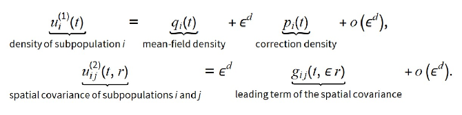
The independent variables t and r respectively denote time and pair-wise distances between individuals (in our case cells). d denotes the dimension of the modelled spatial domain and is a scaling parameter, where L denotes a typical interaction length scale. Note that when L→∞, the SCM density equation reduces to the mean-field equation. The terms can be omitted in practical applications.
Deriving the expressions for q, p, and g , for some biological system of interest, is generally a mathematically cumbersome task. However, Cornell et al. (2019) developed a Wolfram Mathematica Library Package that automates the generation of q, p and g for any biological system that can be expressed by one or more reactant-catalyst-product (RCP) processes. In such RCP-processes,
• reactants are individuals (here cells) that are are consumed in the process,
• catalysts catalyse the process (without getting consumed in it),
• products are produced in the process.
Cell division can, for example, be described by one catalyst (the mother cell) and one product (the daughter cell).
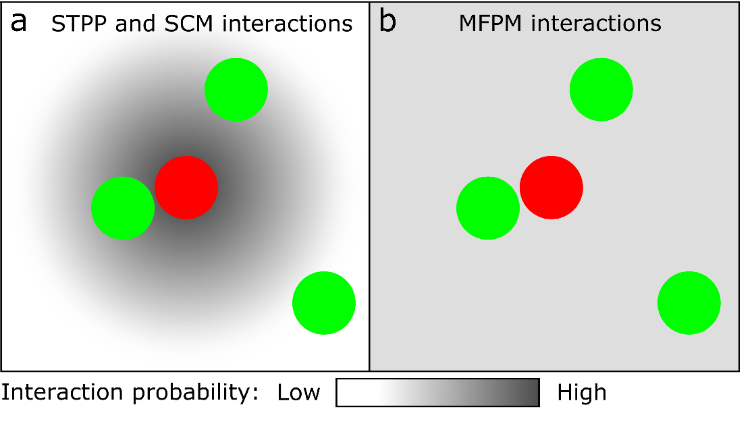
In STPPs and SCMs, the rate (probability per time unit) that two individuals (cells) interact with each other is described by interaction kernels that are functions of pair-wise distances between cells. In the figure below, for example, the focal red cell is more likely to interact with nearby green cells than with faraway green cells (a). In MFPMs, on the other hand, any focal cell is equally likely to interact with all other cells in the system (b).
ϵ=1/L
o()
d
ϵ
Deriving the expressions for q, p, and g , for some biological system of interest, is generally a mathematically cumbersome task. However, Cornell et al. (2019) developed a Wolfram Mathematica Library Package that automates the generation of q, p and g for any biological system that can be expressed by one or more reactant-catalyst-product (RCP) processes. In such RCP-processes,
• reactants are individuals (here cells) that are are consumed in the process,
• catalysts catalyse the process (without getting consumed in it),
• products are produced in the process.
Cell division can, for example, be described by one catalyst (the mother cell) and one product (the daughter cell).
In STPPs and SCMs, the rate (probability per time unit) that two individuals (cells) interact with each other is described by interaction kernels that are functions of pair-wise distances between cells. In the figure below, for example, the focal red cell is more likely to interact with nearby green cells than with faraway green cells (a). In MFPMs, on the other hand, any focal cell is equally likely to interact with all other cells in the system (b).
2. Model
2. Model
We model a cancer system that consists of two cell subpopulations: growth factor producer-cells red) and non-producer-cells ( green). The cells need growth factors in order to divide. As illustrated in the above figure, producer-cells can internalise growth factors produced by themselves (a) or by other producer-cells (b). Non-producer-cells must receive growth factors from producer-cells in order to divide (c). The size of the plus-sign indicates the benefit, in terms of proliferation rate, that a cell gains from a depicted cell-cell interaction. Note that it is beneficial for cells to “free-load” on external growth factors, because then they do not need to spend energy on growth-factor production. Additionally, if drugs are applied to the system, the cells may die. This cancer system can be compactly described by five reactant-catalyst-product (RCP) processes:
(subpopulation,
s
1
subpoulation
s
2,

Biologicalprocess | Reactants(r),catalysts(c),products(p). | Description |
Birth[ s 1 B 1 x 1 x 2 | r=⌀,c={ x 1, s 1 x 2, s 1 | Acellwithmark s 1 x 1 s 1 x 2 B 1 x 1 x 2 |
BirthByFacilitation[ s 1 s 1 B 11 x 1 x 2 x 1 x 3 | r=⌀,c={{ x 1, s 1 x 3, s 1 x 2, s 1 | Acellwithmark s 1 x 1 s 1 x 2 B 11 x 1 x 2 s 1 x 3 x 1 x 2 |
BirthByFacilitation[ s 2 s 1 B 12 x 1 x 2 x 1 x 3 | r=⌀,c={{ x 1, s 2 x 3, s 1 x 2, s 2 | Acellwithmark s 2 x 1 s 2 x 2 B 11 x 1 x 2 s 1 x 3 x 1 x 2 |
DensityIndependentDeath[ s 1 δ 1 | r={ x 1, s 1 | Acellwithmark s 1 x 1 δ 1 |
DensityIndependentDeath[ s 2 δ 2 | r={ x 1, s 2 | Acellwithmark s 2 x 1 δ 2 |
We are going to investigate and density dynamics resulting from three different initial cell configurations (ICCs). These are shown in the left-most column in the figure below. Note that the number of and cells are the same in ICCs 1, 2 and 3. For each investigated ICC, snapshots from one STPP-generated cell population is shown at time points 0, 100 and 200 Δt below.
s
1
s
2
s
1
s
2
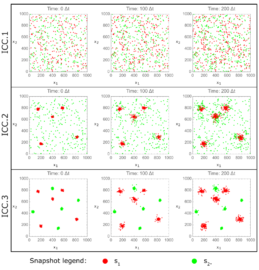
Since the cell-cell interactions are localised in space via interaction kernels, STPP-generated density dynamics depend on the spatial structure of the cell populations. As such, the density dynamics resulting from ICCs 1, 2 and 3 are notably different. On the other hand, MFPM-generated density dynamics resulting from ICCs 1, 2 and 3 all will be the same (since MFPMs are not spatially resolved).
3. Implementation
3. Implementation
3.1 Import Wolfram Mathematica Libraries
3.1 Import Wolfram Mathematica Libraries
To formulate SCMs, we import the following libraries developed by Cornell et al. (2019):
In[]:=
Get["SSPPlibraryOfProcesses`"]
In[]:=
Get["SSPPanalyticalExpressions`"]
3.2 Define the reactant-catalyst-product processes for the modelled system
3.2 Define the reactant-catalyst-product processes for the modelled system
We then define the modelled system in terms of the RCP-processes that are tabulated in the Model description.
Note: To see a list of all pre-defined RCP-processes included in the imported libraries, use the command: ?SSPPlibraryOfProcesses`*
Note: To see a list of all pre-defined RCP-processes included in the imported libraries, use the command: ?SSPPlibraryOfProcesses`*
In[]:=
rcpProcesses={Birth[1,b1,B1,1],BirthByFacilitation[1,1,h,H,b11,B11,1],BirthByFacilitation[2,1,h,H,b12,B12,1],DensityIndependentDeath[1,d1,1],DensityIndependentDeath[2,d2,1]};
3.3 Define variable names and helpful substitutions
3.3 Define variable names and helpful substitutions
We define variable names and substitutions that will simplify both analytical and numerical calculations further down in the Notebook:
In[]:=
qpgVariables={q,p,g};kVariableInG=k;variableOfIntegrationFT=k;xVariableInG=x;variableOfIntegration=x;dim=2;
In[]:=
listOfNumericalSubs={q[1]q1[t],q[2]q2[t],p[1]p1[t],p[2]p2[t],g[1,1,k]G11[t,k],g[1,2,k]G12[t,k],g[2,2,k]G22[t,k],B1[0]totIntB1,B11[0]totIntB11,B12[0]totIntB12,H[0]totIntH};
In[]:=
listOfWSubs=2πktotIntB11G11[t,k]H[k]k->W11[t],2πktotIntB12G12[t,k]H[k]k->W12[t];
∞
∫
0
∞
∫
0
In[]:=
listOfAnalyticalSubs={q1[t]q1,q2[t]q2,p1[t]p1,p2[t]p2,d->2,W11[t]->W11,W12[t]->W12};
Above, we have introduced the functions W11 and W12 in order to (further down) separate terms that will be numerically calculated in real space, from those that will be calculated in Fourier space.
3.4 Generate equations that describe density and spatial covariance dynamics
3.4 Generate equations that describe density and spatial covariance dynamics
Here, G is the Fourier-transform of g, and k is the independent variable in Fourier space.
3.5 Find the death rates that stop the subpopulation densities from increasing
3.5 Find the death rates that stop the subpopulation densities from increasing
We then solve for the MFMP-informed death rates:
And we solve for the SCM-informed death rates:
In the full code project associated with our research article, these death rates are applied to STPPs at the treatment time T (in a C code). For each STPP-generated cancer cell population, we thus measure the quantities q1(T), q2(T), W11(T) and W12(T). By setting the correction densities p1(T) and p2(T) to zero, and working with known model constants, we can thus calculate numerical values for d1(T) and d2(T). We do this for both MFPM and SCM informed death rates.
3.6 Assign numerical model parameter values
3.6 Assign numerical model parameter values
We now assign numerical values to the constant model parameters. We use Gaussian interaction kernels, with integrals and standard deviations labeled with prefixes “totInt” and “σ” respectively.
The model parameters pertaining to cell division are:
And the model parameters pertaining to cell-cell communication via growth factors are:
For simplicity, we gather all kernel rules:
Before drugs are applied to the system, the model parameters pertaining to cell death are:
Lastly, we define the model parameters that pertain to scaling and STPP sampling:
Here, tmin and tmax denote the start and end time of the simulation. The modelled spatial domain is a square with side qside. Minimum and maximum cell-cell separation values are given by rmin and rmax, where rmax=qside/2, as we are using periodic boundary conditions. Cell-cell separations are, moreover, sampled from STPPs with a spatial bin-size rbin. kmin and kmax denote the minimum and maximum value of the independent variable in Fourier space.
3.7 Choose the initial cell configuration
3.7 Choose the initial cell configuration
We choose the ICC that we wish to use. The possible options are 1, 2 or 3 (see the last figure in Notebook Section 2) :
3.8 Import STPP density and spatial covariance data
3.8 Import STPP density and spatial covariance data
STPP dynamics resulting from the three regarded ICCs are simulated in a C-based code. In this Notebook, data describing such STPP dynamics are simply imported from files.
Note that the STPP is stochastic and can, for a given ICC, generate an ensemble of different spatio-temporal point patterns (cell configurations). We therefore import the minimum, mean and maximum density data from 100 STPP simulations per ICC. These files describe the density dynamics when no when no drugs/cell deaths are applied to the system:
In preparation for plotting, we then interpolate the minimum and maximum density data:
We next import the spatial covariance data for the investigated ICC:
3.9 Set the SCM and MFPM initial conditions from the imported STPP data
3.9 Set the SCM and MFPM initial conditions from the imported STPP data
The initial conditions for q (densities) and g (spatial covariances) are set from the imported data. The initial correction values p1(0) and p2(0) are set to zero. Note that the initial conditions g(t,r) must be Fourier-transformed (or, more specifically, Hankel-transformed in our case with d=2 and radial symmetry) to form G(t,k), in accordance with the generated SCM equations.
3.10 Solve the SCM and MFPM equations numerically
3.10 Solve the SCM and MFPM equations numerically
In preparation for the numerical calculations, we define the model rate equations using the previously obtained expressions for Hq1, Hq2, Hp1, Hp2, HG11, HG12, HG22 and the initial conditions:
We are now ready to define a function that numerically calculates q, p and g (or rather, G):
And with the following command, we can now obtain q, p and G:
4. Visualise Results
4. Visualise Results
We visualise density dynamics generated by the STPP, MFPM and SCM in three different plots (4.1-4.3). To allow for visual comparison, we then overlay the plots in 4.4.
4.1 Generate the STPP density dynamics plot (pre-drug)
4.1 Generate the STPP density dynamics plot (pre-drug)
4.2 Generate the MFPM density dynamic plots (pre-drug)
4.2 Generate the MFPM density dynamic plots (pre-drug)
4.3 Generate the SCM density dynamic plots (pre-drug)
4.3 Generate the SCM density dynamic plots (pre-drug)
4.4. Overlay the density dynamic plots for visual model comparisons (pre-drug)
4.4. Overlay the density dynamic plots for visual model comparisons (pre-drug)
4.5 Results presented in the original research article
4.5 Results presented in the original research article
In the original research article, we show that SCMs can capture STPP-generated population density dynamics, even when mean-field population models (MFPMs) fail to do so. As can be seen in the figure below, for ICC.1, both the MFPM and the SCM capture STPP density dynamics. However, for ICCs 2 and 3, the SCM captures STPP density dynamics whereas the MFPM does not.
You can verify this by changing the variable “ICCoption” in 3.7!
You can verify this by changing the variable “ICCoption” in 3.7!
We also show that SCM-informed treatment strategies outperform MFPM-informed strategies in terms of inhibiting population growths. Following the procedure outlined in 3.5, drugs are applied at time T=200Δt in the STPP. The resulting density dynamics are shown in the figure below, in which each track corresponds to one spatio-temporal point pattern (STPP-generated cancer cell population).
5. Significance and Concluding Remarks
5. Significance and Concluding Remarks
Due to the pre-clinical and clinical applications of mathematical oncology models (Rockne et al., 2019), there exists a need to formulate analytical cancer models that capture localised cell-cell interactions, maintain cell discreteness and are spatio-temporal. In this work, we suggested using spatial cumulant models (SCMs) to achieve this.
Deriving SCMs for a specific biological system can be a mathematically challenging and cumbersome task. However, using a Wolfram Mathematica Library Package, the generation of SCMs can be automated for a broad family of biological systems (more specifically any system that can be described in terms of reactant-catalyst-product processes).
In this Notebook, we used Wolfram Mathematica to
(1) generate SCMs and MFPMs that describe our regarded cancer system,
(2) analytically derive spatially informed treatment strategies via SCMs (and non-spatially informed treatment strategies via MFPMs),
(3) numerically solve the SCM and MFPM equations,
(4) visually compare the resulting STPP, SCM and MFPM density dynamics.
We anticipate that the opportunity to analytically derive spatially informed cancer treatment strategies, as enabled via SCMs, will inspire new theoretical and applied research ventures.
References
References
S. J. Cornell, Y. F. Suprunenko, D. Finkelshtein, P. Somervuo, and O. Ovaskainen. A unified framework for analysis of individual-based models in ecology and beyond. Nat Commun, 10(1):4716, 10 2019. doi: https://doi.org/10.1038/s41467-019-12172-y.
O. Ovaskainen, D. Finkelshtein, O. Kutoviy, S. Cornell, B. Bolker, and Y. Kondratiev. A general mathematical framework for the analysis of spatiotemporal point processes. Theor Ecol, 7:101–113, 2014. doi: https://doi.org/10.1007/s12080-013-0202-8.
R. C. Rockne, A. Hawkins-Daarud, K. R. Swanson, J. P. Sluka, J. A. Glazier, P. Macklin, D. A. Hor- muth, A. M. Jarrett, E. A. B. F. Lima, J. Tinsley Oden, G. Biros, T. E. Yankeelov, K. Curtius, I. Al Bakir, D. Wodarz, N. Komarova, L. Aparicio, M. Bordyuh, R. Rabadan, S. D. Finley, H. En- derling, J. Caudell, E. G. Moros, A. R. A. Anderson, R. A. Gatenby, A. Kaznatcheev, P. Jeavons, N. Krishnan, J. Pelesko, R. R. Wadhwa, N. Yoon, D. Nichol, A. Marusyk, M. Hinczewski, and J. G. Scott. The 2019 mathematical oncology roadmap. Phys Biol, 16(4):041005, 06 2019. doi: https://doi.org/10.1088/1478-3975/ab1a09.
CITE THIS NOTEBOOK
CITE THIS NOTEBOOK
Spatial cumulant models for local interactions in cancer systems
by Sara Hamis
Wolfram Community, STAFF PICKS, June 28 2022
https://community.wolfram.com/groups/-/m/t/2559644
by Sara Hamis
Wolfram Community, STAFF PICKS, June 28 2022
https://community.wolfram.com/groups/-/m/t/2559644