What is a Variational Quantum Eigensolver (VQE)?
What is a Variational Quantum Eigensolver (VQE)?
VQEs use both classical and quantum computing to solve for the ground state of a given Hamiltonian, an operator which gives the energy of a system. Once the Hamiltonian is determined, one must determine an appropriate ansatz. A VQE ansatz is typically composed of a series of parametrized gates on a quantum circuit. These gates are initialized to the zero state, but with cumulative modification to the parameters, will ideally give the ground state of the Hamiltonian. Next, all VQEs use some sort of classical minimization routine. Here I will use Mathematica’s NMinimize, which automatically determines an optimal routine for the problem and numerically searches for the global minimum. The quantum computing component to VQE is the cost function of this routine. The cost function takes in a list of parameters and the desired ansatz, computes the quantum state, and outputs the expectation value of this state with respect to the Hamiltonian. With enough iterations, a good minimization routine, and a good ansatz, we should be able to find the exact ground state of the system along with its corresponding energy.
Defining Helper Functions
Defining Helper Functions
Below are several functions necessary for computing the ground state energy via VQE:
◼
expectationValue: computes the expectation value of a quantum state with respect to a quantum operator
In[]:=
expectationValue[hamiltonian_QuantumOperator,state_QuantumState]:=QuantumCircuitOperator[{state,hamiltonian,state["Dagger"]}][]
◼
harcoreBoseHubbardHamiltonian: a quantum operator that describes interacting bosonic particles confined to a one-dimensional lattice. Taking its expectation value with a quantum state in the computational basis gives the energy of the state. Its kinetic energy describes boson mobility in the lattice and is scaled by the hopping amplitude (t). Its potential energy is defined as the number of particles all sites and is scaled by the chemical potential (μ). The number of sites, t and μ are all user defined inputs, however I am choosing to set t = μ = 1.
In[]:=
hardcoreBoseHubbardHamiltonian2[sites_,t_:1,μ_:1]:=(-t/2)Total[Table[QuantumOperator["XX"+"YY",{i,i+1}],{i,1,sites-1}]]+(-μ/4)Total[Append[Table[-1*QuantumOperator["Z",{i}],{i,1,sites}],2*sites]]hardcoreBoseHubbardHamiltonian1[sites_,t_:1,μ_:1]:=Flatten[{(-t/2)Table[QuantumOperator["XX"+"YY",{i,i+1}],{i,1,sites-1}],(-μ/4)Append[Table[-1*QuantumOperator["Z",{i}],{i,1,sites}],2*sites*QuantumOperator[StringRepeat["I",sites]]]}]hardcoreBoseHubbardHamiltonian[sites_,t_:1,μ_:1]:=Flatten[{(-t/2)Table[{QuantumOperator["XX",{i,i+1}],QuantumOperator["YY",{i,i+1}]},{i,1,sites-1}],(-μ/4)Append[Table[-1*QuantumOperator["Z",{i}],{i,1,sites}],2*sites*QuantumOperator[StringRepeat["I",sites]]]}]
◼
evolveRotateAnsatz: this parametrized ansatz circuit consists of a specified number of repetitions of Hamiltonian evolution gates followed by single qubit rotation gates about the Z and Y axes. It is preferred for analog quantum computing hardware (i.e. ultracold bosons in optical lattices) due to being able to exactly simulate the Hamiltonian evolution. To implement the ansatz as on a quantum circuit as is done here, the non-unitary Hamiltonian evolution gate must be approximated as the composition of unitary gates via Trotterization.
In[]:=
evolveRotateAnsatz[hamiltonian_,sites_,layers_,θ_]:=(*num_params=1+layers(2sites+1)*)(evolve=QuantumCircuitOperator[{"Trotterization",hamiltonian,1,1,#}]&;rzLayer=MapIndexed[{"RZ",#1}->#2&,{##}]&;ryLayer=MapIndexed[{"RY",#1}->#2&,{##}]&;circuit=QuantumCircuitOperator[Flatten[{Table[{evolve@@θ[[1+i(2*sites+1)]],rzLayer@@θ[[2+i(2sites+1);;1+sites+i(2sites+1)]],ryLayer@@θ[[2+sites+i(2sites+1);;1+2sites+i(2sites+1)]]},{i,0,layers-1}],evolve@@θ[[1+layers(2sites+1)]]}]];circuit)
◼
twoLocalAnsatz: this parametrized ansatz circuit consists of a specified number of layers of single qubit rotations about the Y axis followed by linearly entangling CNOT gates. It is preferred for digital quantum computing hardware since it is exclusively composed of unitary operations, and thus is mappable to a quantum circuit without need for approximation.
In[]:=
twoLocalAnsatz[sites_,layers_,θ_]:=(*num_params=sites*(layers+1)*)(cnotLayer=Map[{"CNOT"}->{#,#+1}&,{##}]&;ryLayer=MapIndexed[{"RY",#1}->#2&,{##}]&;circuit=QuantumCircuitOperator[Flatten[{Table[{ryLayer@@θ[[1+i(sites);;(i+1)(sites)]],cnotLayer@@Range[1,sites-1]},{i,0,layers-1}],{ryLayer@@θ[[1+layers*sites;;(layers+1)*sites]]}}]];circuit)
◼
cost: this is the cost function to be fed into the minimization routine. It takes in a list of parameters and the desired ansatz, computes the quantum state, and outputs the expectation value of this state with respect to the Hamiltonian.
In[]:=
cost[θ_,ansatz_,hamiltonian_]:=Module[{state},If[ansatz=="evolveRotateAnsatz",state=evolveRotateAnsatz[hamiltonian,sites,layers,θ][],If[ansatz=="twoLocalAnsatz",state=twoLocalAnsatz[sites,layers,θ][]]];exp=Re[expectationValue[Total[hamiltonian],state]["Scalar"]];Simplify[exp,Assumptions->x[_]∈Reals]]
Define VQE Function
Define VQE Function
In[]:=
VQE[sites_,layers_,hamiltonian_,ansatz_]:=Module[{nparams},If[ansatz=="evolveRotateAnsatz",nparams=1+layers(2sites+1),If[ansatz=="twoLocalAnsatz",nparams=sites*(layers+1)]];expr=cost[Array[x,nparams],ansatz,hamiltonian];solution=NMinimize[{expr,And@@Table[0<=x[i]<=2*Pi,{i,nparams}]},Array[x,nparams]];{solution,expr}]
Takes the number of sites, number of layers, Hamiltonian quantum operator, and parametrized ansatz circuit as an input. The first output is the solution, which is a list containing the computationally predicted ground state energy, and the circuit parameters which give the ground state. The second output is the symbolic expression for the energy of a state given by the specified ansatz and Hamiltonian.
Sites = 1
Sites = 1
Lets start with the most basic case: a single qubit.
In[]:=
sites=1;ham=hardcoreBoseHubbardHamiltonian[sites,1,1];Total[ham]
Out[]=
--
|0〉〈0|
4
3(|1〉〈1|)
4
In[]:=
Print["The true ground state energy is ",N[Min[Eigenvalues[Total[ham]["Matrix"]]]]]
The true ground state energy is -0.75
evolveRoteAnsatz, layers = 1
evolveRoteAnsatz, layers = 1
In[]:=
layers=1;ansatz="evolveRotateAnsatz";evolveRotateAnsatz[ham,sites,layers,Array[x,layers(2sites+1)+1]]["Diagram"]
Out[]=

In[]:=
{soln11er,expr11er}=VQE[sites,layers,ham,ansatz]
Out[]=
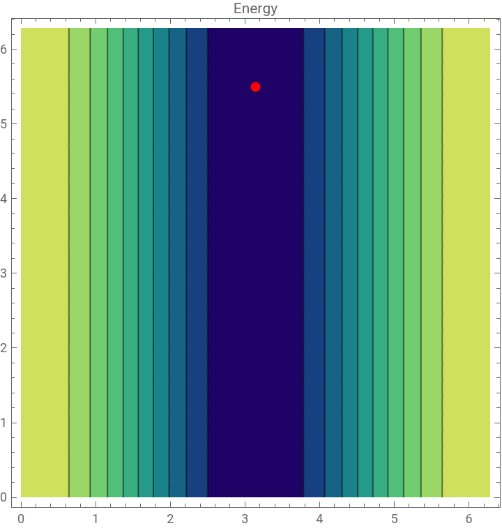
{-0.75,{x[1]4.20596,x[2]4.13558,x[3]3.14159,x[4]5.4947}},(-4+Re[+])
1
8
-x[3]
x[3]
1 layer of the evolve-rotate Ansatz is sufficient to reach the exact ground state energy: -0.75
In[]:=
ContourPlot[Evaluate[expr11er/.soln11er[[2]][[{1,2}]]],{x[3],0,2Pi},{x[4],0,2Pi},Epilog->{Red,PointSize[Large],Point[Values[soln11er[[2]]][[{3,4}]]]},ColorFunction->"BlueGreenYellow",PlotLegends->Automatic,PlotLabel->"Energy"]
Out[]=

twoLocalAnsatz, layers = 1
twoLocalAnsatz, layers = 1
1 layer of the two-local Ansatz is sufficient to reach the exact ground state energy : -0.75
From both plots it is evident that the ground state can be achieved with a single rotation about the Y axis.
Sites = 2
Sites = 2
Next, a slightly less trivial case.
Layers = 1, evolveRotateAnsatz
Layers = 1, evolveRotateAnsatz
1 layer of the evolve-rotate Ansatz is 0.375 away from the true ground state energy.
NMinimize did its best given the ansatz. However the ansatz simply does not allow for the freedom to reach the ground state of the system.
Layers = 1, twoLocalAnsatz
Layers = 1, twoLocalAnsatz
1 layer of the two-local Ansatz is sufficient to reach the exact ground state energy for 2 sites : -2
Since there are 4 independent parameters determining the energy of the ground state, we can create 4 different 3D diagrams by fixing a different parameter each time.
Plotting
Plotting
All of the 3D density plots above confirm that the VQE has successfully optimized all parameters to give the ground state.
Layers = 2, evolveRotateAnsatz
Layers = 2, evolveRotateAnsatz
2 layers of the evolve-rotate Ansatz is 0.17379 away from the exact ground state energy.
Since there are 9 independent parameters determining the energy of the ground state, we could create several different 3D diagrams by fixing different parameters each time.
Instead I will just show you the 2 most interesting ones.
Instead I will just show you the 2 most interesting ones.
Generating and Storing Plot Data
Generating and Storing Plot Data
Plotting
Plotting
The 3D density plots above confirm that the optimization routine has reached the minimum energy possible given the ansatz, though the exact ground state has not been reached. More layers would be required for better accuracy.
Sites = 3
Sites = 3
It starts to take quite long to run with 3 sites, so we will just consider the case of 1 layer using the two-local ansatz.
Layers = 1, twoLocalAnsatz
Layers = 1, twoLocalAnsatz
1 layers of the two-local Ansatz is 0.27336 away from the ground state energy.
Since there are 6 independent parameters determining the energy of the ground state, we could create several different 3D diagrams by fixing different parameters each time.
Instead I will just show you the 2 most interesting ones.
Instead I will just show you the 2 most interesting ones.
Plotting
Plotting
NMinimize did its best given the ansatz. However the ansatz simply does not allow for the freedom to reach the ground state of the system.
Concluding Remarks
Concluding Remarks
Why Use VQE?
Why Use VQE?
Challenges and Improvements
Challenges and Improvements
The max number of parameters we dealt with was 11, in the 2 sites 2 layers case using the evolve-rotate ansatz. Cases more ambitious than this simply took too long to run. Yet, the VQE is evaluating significantly faster than it was initially, since improvements were made such as numerical optimization (as opposed to symbolic) and harnessing the efficiency of tensor contraction built into the Quantum Framework. However, I am confident further speedup could be achieved, most likely pertaining to the minimization routine. Further the 1D Hardcore Bose-Hubbard Hamiltonian is just one of countless Hamiltonians that could be solved via VQE. If time permitted, I would have tested out many more Hamiltonians and added more ansatz functionalities to compliment them.
Acknowledgements
Acknowledgements
Big thanks to my mentors Nik and Mano for inspiring a deeper intuition and passion for quantum computing, and writing good Mathematica code. Thanks to Josh for giving me tips for creating aesthetically pleasing plots. Thanks to Steven Wolfram for sharing with me his wisdom on the value and drawbacks of quantum computing. Lastly, thanks to everyone else who taught me something and/or made the last couple weeks lots of fun.
CITE THIS NOTEBOOK
CITE THIS NOTEBOOK
Developing a variational quantum eigensolver
by Arielle Sanford
Wolfram Community, STAFF PICKS, July 13, 2023
https://community.wolfram.com/groups/-/m/t/2959959
by Arielle Sanford
Wolfram Community, STAFF PICKS, July 13, 2023
https://community.wolfram.com/groups/-/m/t/2959959