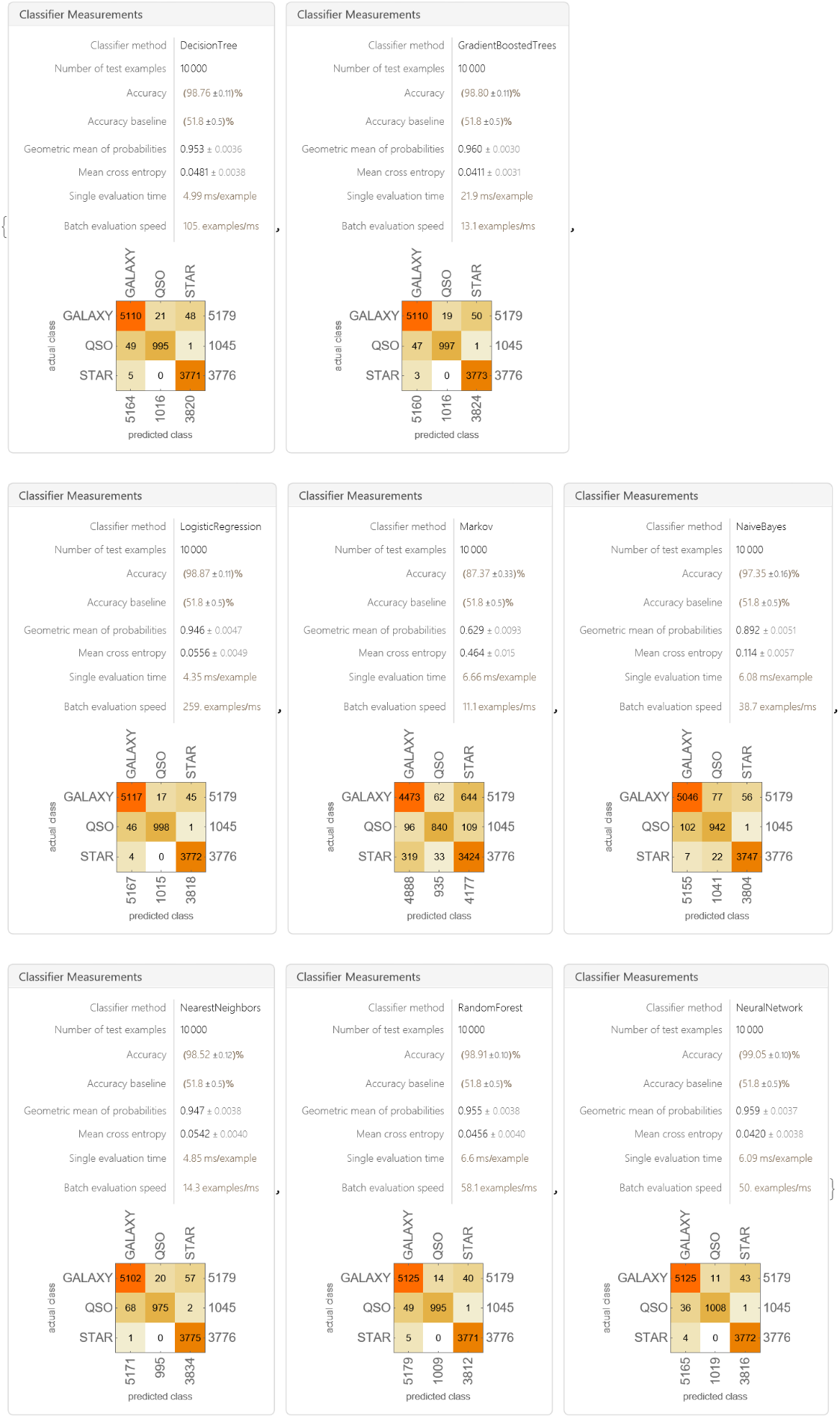
Distinguishing astronomical source types is straightforward with available spectroscopical and multi-wavelength observations data, but obtaining detailed observations for millions of celestial objects is time-consuming and impractical with the rates at which current telescopes generate data. In contrast, classifying sources with only photometry in multiple wavebands is comparatively fast, and with machine learning involved, even more rapid classification of the data can be performed. Work done in this project involves the classification of galaxies, stars, and quasars with different machine learning methods, comparing them, and exploring and analyzing data from the dataset containing photometric observations of celestial objects; The classification achieved astonishing accuracy of 99.05% with neural networks and analysis of data shows very clear correlation patterns for each class.
Machine learning with SDSS dataset
Machine learning with SDSS dataset
◼
Data was taken from Data Release 16 (DR16) of Sloan Digital Sky Survey (SDSS) which can be obtained from here.
In[]:=
s=SemanticImport["C:\\Users\\Deep\\Downloads\\SDSS\\Skyserver_data.csv"]
Out[]=
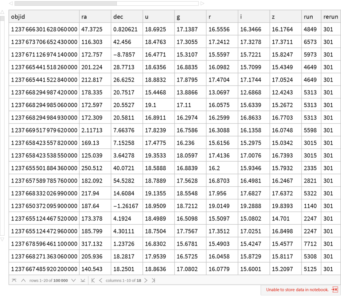
Structure of the Dataset
Structure of the Dataset
◼
Missing value count was found across each with Count[_Missing]
In[]:=
Grid[{{"objid","ra","dec","u","g","r","i","z","run","rerun","camcol","field","specobjid","class","redshift","plate","mjd","fiberid"},s[Count[_Missing],#]&/@{"objid","ra","dec","u","g","r","i","z","run","rerun","camcol","field","specobjid","class","redshift","plate","mjd","fiberid"}},Frame->All]

◼
Unique value count was found with CountDistinct
In[]:=
Grid[{{"objid","ra","dec","u","g","r","i","z","run","rerun","camcol","field","specobjid","class","redshift","plate","mjd","fiberid"},CountDistinct@s[All,#]&/@{"objid","ra","dec","u","g","r","i","z","run","rerun","camcol","field","specobjid","class","redshift","plate","mjd","fiberid"}},FrameAll]

Detected photometric objects are enumerated within a given imaging field. Thus, multiple fields may have objects with the same object number. But looking at the specobjid, it can be seen that there are 100,000 unique spectras, meaning there should be 100,000 unique objects.
In[]:=
BarChart[s[Count[#],"class"]&/@{"STAR","GALAXY","QSO"},ChartLabels{"Star","Galaxy","Quasars"},AxesLabel{"","Count"},ChartStyle{Red,Orange,Yellow}]
◼
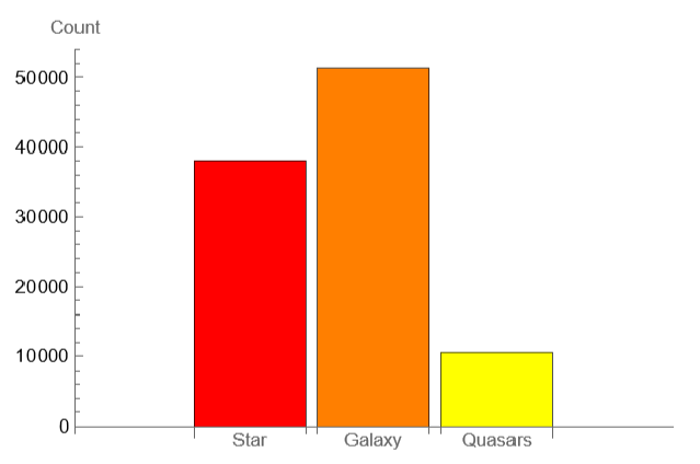
We can see here that we have 4-5 times more galaxies and stars compared to quasars, meaning that ML models would be a little less accurate in being able to predict quasars due to the low number of samples.
Taking relevant data for training machine learning models
Taking relevant data for training machine learning models
◼
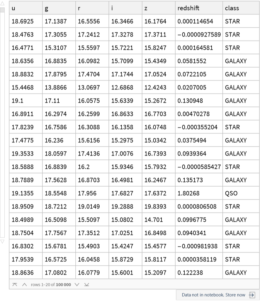
Some of these columns are here mostly for keeping track of the images such as objid and specobjid. Objid and Specobjid are made of the other features camcol, field, mjd, plate, fiberid, run, and rerun; these features describe telescope movement and Image processing . These features do not really describe the star, galaxy, or quasar which means these features can be removed for training the dataset. It is also relevant to drop RA and Dec because, these are the celestial coordinates and celestial bodies can’t be classified based on their location in space as they are all equally probable.
In[]:=
data=s[All,{4,5,6,7,8,15,14}]
Out[]=
Creating training and test datasets and classification with classify
Creating training and test datasets and classification with classify
◼
Creating training set of 90% of complete dataset and 10% of remaining will be test set
In[]:=
{ctrain,ctest}=TakeDrop[RandomSample[data],90000];
In[]:=
{a,b,c,d,e,f,g,h}=Classify[ctrain->"class",Method#]&/@{"DecisionTree","GradientBoostedTrees","LogisticRegression","Markov","NaiveBayes","NearestNeighbors","RandomForest","NeuralNetwork"};
Evaluating performance of ML models
Evaluating performance of ML models
After the training we will make an evaluation of the model and measuring its performance . For that, we will try different metrics as :
◼
Classifier Measurements(contains accuracy and confusion matrix plot)
◼
Calibration Curve : Plot between actual and predicted probabilities of the classifier.
◼
Area under ROC Curve: It tells how much model is capable of distinguishing between classes.
In[]:=
ClassifierMeasurements[#,ctest]&/@{a,b,c,d,e,f,g,h}
Out[]=
Plotting Calibration Curves
Plotting Calibration Curves
Area under ROC curve
Area under ROC curve
Feature Importance with SHapley Additive exPlanations(SHAP Values)
Feature Importance with SHapley Additive exPlanations(SHAP Values)
◼
Random 500 values from test dataset(ctest) are used with DecisionTree to get corresponding SHAP Values
◼
It can be clearly see how important is redshift in predicting stars and galaxies! this is just for DecisionTree, for other models these results would vary.
◼
following are the results for a particular value(z) in test dataset (ctest) for different models
Exploratory data analysis with the dataset
Exploratory data analysis with the dataset
Velocity and distance of the celestial body
Velocity and distance of the celestial body
Since recessional velocity can be found out with redshift, by Hubbles law proper distance can be found out
Bottom row of above grid is the redshift of the corresponding object
Feature vs count plot and distribution chart for different class of objects
Feature vs count plot and distribution chart for different class of objects
◼
Distribution Chart
Correlation between features
Correlation between features
Above plot clearly shows the separation of all three classes of the objects.
◼
Sky Coverage:
The curves in above list plot are the scanning runs performed by the telescope showing stripes, according to information available at SDSS sky coverage, these stripes are 2.5 degrees wide and each strip has a number associated with it.
Concluding remarks
Concluding remarks
Accuracy of 99.05% achieved by neural net is certainly remarkable, but it can be further improved by tweaking the ML models, also the visual exploration of this dataset also revels plenty of patters raising lot of questions and answers .Further exploration could lead to finding anomalies in the dataset meaning it could give us some interesting results and opening up the possibility of future research.
Keywords
Keywords
◼
Machine Learning
◼
SDSS
◼
Astronomy
Acknowledgment
Acknowledgment
I’d like to thank my mentor Dr. Sotiris Michos for guiding me throughout project , he reviewed my project at every step and suggested changes to improve it and also to all the TA’s for helping me out whenever needed.
References
References