This project implements a visualization tool to explore the dynamic evolution of geopolitical borders over historical ranges. By taking traditional 2D historical maps and stacking them along a vertical time axis, we can obtain a continuous 3D spacetime volume, offering a clear perspective on the trajectory of historical entities.
Introduction
Introduction
When studying History, we rely on maps to understand the territorial reach of empires, kingdoms, and republics. However, traditional cartography is constrained by its two-dimensional nature: a standard map can only represent the borders of an empire at a single moment in time. While interactive timelines can show how borders change, they force the observer to view history frame by frame, without the corresponding sense of continuity when it comes to understanding a historical period.
To overcome this limitation, this essay explores a computational approach that treats time as a physical third dimension. In this setup, a historical country becomes a 3D shape, making it easier to spot territorial expansions, periods of stability, or sudden collapses at a single glance.
In the following sections, we will build a step-by-step computational pipeline. We will query dated territorial polygons, align different historical eras onto a normalized canvas, and interpolate the gaps between available dates. Finally, we will render these frames into an interactive 3D plot that lets us explore geopolitical history from a spatio-temporal perspective.
Data Acquisition
Data Acquisition
Wolfram History Database
Wolfram History Database
The Wolfram Language has access to an extensive collection of historical data. Specifically, the HistoricalCountry Entity, includes sovereign powers, empires, culturally similar independent states, and many other forms of countries across History. Multiple data can be retrieved from a historical country entity, such as its area, start and end dates, etc.
Extract all available information from the Second Spanish Republic in a Dataset form:
In[]:=
Out[]=
|
Data Recovery
Data Recovery
Since the HistoricalCountry Entity contains information about the current countries they spanned, it is straightforward to select a current country and get a list of all the empires and powers that at some point were based in the country selected.
Get a list of entities that took place at the current Italy, sorted by the end date:
In[]:=
SortBy[EntityList[EntityClass["HistoricalCountry","CurrentCountries"->Entity["Country","Italy"]]],#["EndDate"]&]//Shallow
Out[]//Shallow=
,,,,,,,,,,88
One important property that most HistoricalCountry Entities contain is “Polygon”. The Polygon of an entity is a representation of the entity’s territory. It can be plotted using GeoGraphics. It is a great starting point, but it only gives us a single static snapshot of the territory, usually at its maximum extent.
Plot the Holy Roman Empire:
In[]:=
GeoGraphicsEdgeForm[Thickness[0.005]],StandardRed,["Polygon"]
Out[]=
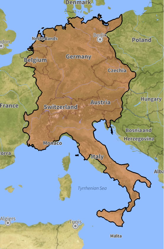
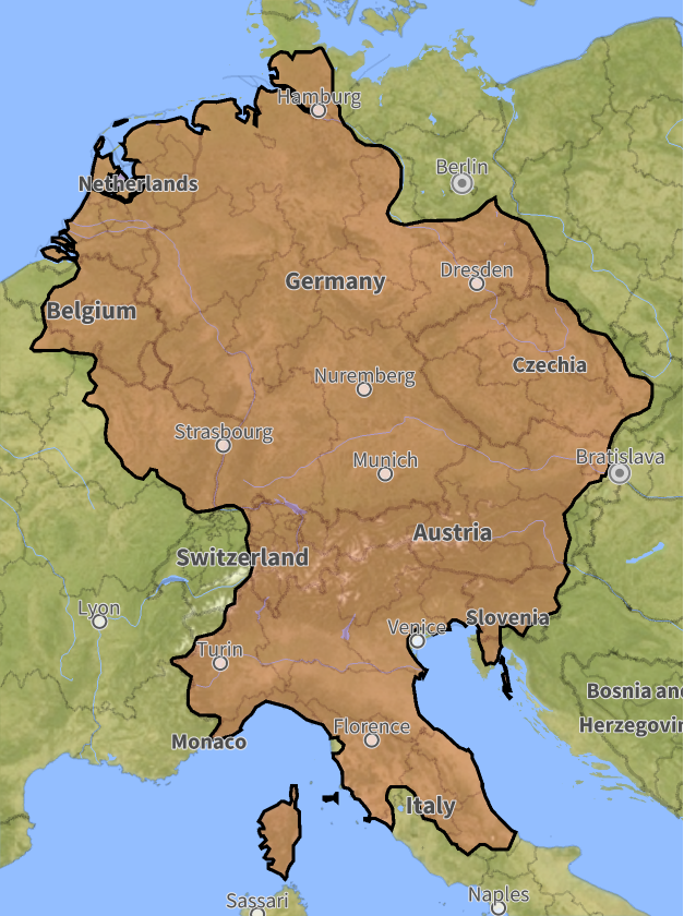
However, borders are rarely static; they expand, contract, and fragment through conquests and treaties. To capture this movement, we can retrieve the polygon of a territory for any specific year just by attaching a date. This enables us to reconstruct a chronological sequence of territorial shapes, forming the discrete frames that we will later interpolate to build our continuous spacetime volume.
Select the polygon of the Holy Roman Empire in the year 1012:
In[]:=
holyRomanEmpire1012=["Polygon","Date"->DateObject[{1012}]];
Plot the Holy Roman Empire in the year 1012:
In[]:=
GeoGraphics[{EdgeForm[Thickness[0.005]],StandardRed,holyRomanEmpire1012}]
Out[]=
Therefore, it is possible for us to define a function that, given a historical country, retrieves all the polygons along with the year for which the Wolfram Database has data.
Get all polygons available of the Inca Empire :
In[]:=
incaFrames=extractHistoricalPolygons
Out[]=
1439,PolygonGeoPosition,1464,PolygonGeoPosition,1471,PolygonGeoPosition,1494,PolygonGeoPosition,1501,PolygonGeoPosition,1526,PolygonGeoPosition

The Challenge of Spatial Alignment
The Challenge of Spatial Alignment
Once we have our sequence of historical polygons, we face an alignment challenge. If we simply plot each polygon using its immediate boundaries, a small state (like Andorra) might occupy the same visual size as a massive empire. When stacked vertically in 3D, this would distort the physical scales completely.
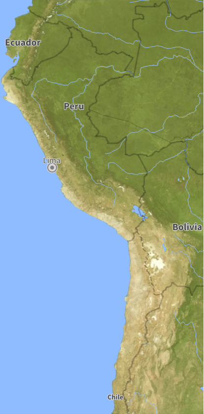
To prevent this misalignment, we must unify the coordinates of each polygon. We use GeoBounds for that purpose, which takes the list of all frames and calculates the smallest boundary that contains all territories in the list.
Get the boundary that contains all the frames of the Inca Empire :
In[]:=
incaBounds=historicalCountryGeoBounds[incaFrames]
Out[]=
{{-32.9865,2.2626},{-81.3208,-64.0723}}
Plot the region in a world map
In[]:=
GeoGraphics[GeoRange->incaBounds]
Out[]=
Constructing the Spacetime Volume
Constructing the Spacetime Volume
Projecting 2D Borders into Time
Projecting 2D Borders into Time
With our spatial standard canvas across all timeframes, we can begin moving from 2D geometry into 3D space. Using the standardized geographic bounds, we convert the vector polygon of each available year into a 2D texture. These textures will be projected onto horizontal 3D rectangular planes, positioning each plane along the vertical z-axis at a height corresponding to its exact historical year. This creates a chronological sequence of floating planes, marking the exact years where territorial data is available in the Wolfram History Database.
Out[]=

Temporal Interpolation via Morphing
Temporal Interpolation via Morphing
A critical challenge in historical data analysis is dealing with temporal gaps. Historical records rarely provide year-by-year boundary updates; therefore, two consecutive data frames might be separated by decades. Simply stacking our discrete planes leaves an empty void space between them.
To fill these gaps, we must generate intermediate frames that simulate how borders evolved during the unrecorded years. In order to accomplish that, we convert our map frames into binary images and compute their signed distance transform. By linearly interpolating across these distance fields, we achieve smooth transitions where borders progressively expand, shrink, or merge across time. For that purpose, we use the function interpolateFrameTransition.
Voxelization and Surface Meshing
Voxelization and Surface Meshing
Once we have computed the sequence of interpolated binary frames, we can stack them using Image3D. This produces a solid voxel grid, which is essentially a collection of discrete blocks . In order to turn it into a smooth sculpture, we use ImageMesh. The result is a continuous geometric surface around the solid boundary.
While the X and Y axes of the generated mesh simply correspond to image width and height, the Z-axis represents internal slice indices rather than the corresponding year. As the data frames are not separated by regular intervals of years, slice indices do not map linearly across the entire timeline. To fix this, we build an interpolation function (trueTransform) that maps each Z-slice index back to its exact historical year. When rendered, this calibrated mesh aligns perfectly with our discrete planes.
While the X and Y axes of the generated mesh simply correspond to image width and height, the Z-axis represents internal slice indices rather than the corresponding year. As the data frames are not separated by regular intervals of years, slice indices do not map linearly across the entire timeline. To fix this, we build an interpolation function (trueTransform) that maps each Z-slice index back to its exact historical year. When rendered, this calibrated mesh aligns perfectly with our discrete planes.
This 3D solid, and the corresponding animation shown above, condense the 95-year history of the Inca Empire into a model that can be rotated and zoomed to visually explore the empire’s expansion.
Case Studies: Reading Geopolitics Through Volumes
Case Studies: Reading Geopolitics Through Volumes
The German Transition : Weimar Republic to Nazi Germany (1918-1945)
The German Transition : Weimar Republic to Nazi Germany (1918-1945)
Generate the combined spacetime volume for both consecutive German regimes:
This case study demonstrates historicalCountrySpacetimePlot’s ability to chain historical eras into a single spacetime volume. The lower section shows the stable borders of the Weimar Republic (1918-1933). The mesh transition into Nazi Germany (1933-1945) is geometrically seamless. However, after 1938, the sculpture undergoes an aggressive horizontal expansion that captures the rapid annexations of World War II before collapsing.
The Byzantine Empire (395 - 1453) : The Slow Erosion
The Byzantine Empire (395 - 1453) : The Slow Erosion
Generate the spacetime volume of the Byzantine Empire:
The Byzantine Empire provides a perfect example of long-term territorial contraction. Instead of a rapid expansion, the resulting 3D geometry resembles an inverted cone. The wide base reflects its massive 6th-century Mediterranean reach, which then undergoes a centuries-long erosion. As time moves upward along the Z-axis, the volume shrinks, showing how the empire was reduced to just the city of Constantinople.
The Macedonian Empire : Rapid Expansion and Instant Fragmentation
The Macedonian Empire : Rapid Expansion and Instant Fragmentation
Plot the Macedonian Empire with lower opacity :
The Macedonian Empire (807-168 BC) offers a striking example of explosive territorial growth. The model starts as a narrow vertical needle centered around Greece. Then, in a short period of time, the geometry expands aggressively to the east, corresponding to Alexander the Great’s rapid conquests through Egypt, Persia, and the borders of India. Finally, the sculpture terminates abruptly at its absolute maximum width, preserving the sudden death of the king and the immediate fragmentation of his realm into the Diadochus Kingdoms.
Concluding Remarks
Concluding Remarks
Current Limitations
Current Limitations
While the pipeline developed reconstructs historical empires and serves as a study tool, a current limitation of the project is its inability to accurately plot contemporary countries.
Future Steps
Future Steps
Following the conclusion of this program, my objective is to correct this modern-country rendering problem, thoroughly document the core functions, and submit the optimized historicalCountrySpacetimePlot to the Wolfram Function Repository.
Looking further ahead, my ultimate goal is to package these tools, along with new ones, into a dedicated HistoryVisualization Paclet to serve as a new educational and research tool.
Looking further ahead, my ultimate goal is to package these tools, along with new ones, into a dedicated HistoryVisualization Paclet to serve as a new educational and research tool.
Acknowledgments
Acknowledgments
Special thanks go to Phileas for his exceptional involvement and dedication to this project. His technical expertise is matched only by his enthusiasm and willingness to turn every doubt into an enriching lecture. My thanks to Eric for his valuable comments and corrections, which made this project much easier to understand and debug. I am also grateful to the team of mentors and to Stephen Wolfram for suggesting this project. Additionally, I would like to thank Stephanie for her outstanding work throughout the program, ensuring that everything ran smoothly. Finally, I want to express my gratitude to the entire WSRI community for making this experience a defining moment that has shaped the person I am striving to become.
References
References
1
.Animate the Rise and Fall of Historical Countries, wolfram.com. Retrieved July, 2026 from https://www.wolfram.com/language/11/knowledgebase-expansion/animate-the-rise-and-fall-of-historical-countries.html.en?footer=lang
AI Disclosure
AI Disclosure
The following generative AI tool was used in this project: Gemini 1.5 Pro. It was used exclusively for brainstorming and studying empires and republics whose evolution deserve to be visualized with this modern tool. All technical code, mathematical formulations, and computational logic were entirely developed, reviewed, and approved by the author without the use of generative AI tools.
CITE THIS NOTEBOOK
CITE THIS NOTEBOOK
Time Is All You Need: A Tubular Representation of Historical Borders
by Alejandro Barranco Pérez
Wolfram Community, STAFF PICKS, July 16, 2026
https://community.wolfram.com/groups/-/m/t/3761669
by Alejandro Barranco Pérez
Wolfram Community, STAFF PICKS, July 16, 2026
https://community.wolfram.com/groups/-/m/t/3761669