CITE THIS NOTEBOOK: Identifying possible observational signatures of spacetime discretization in strongly relativistic astrophysical phenomena by Vittoria Tommasini. Wolfram Community JAN 13 2023.
CITE THIS NOTEBOOK: Identifying possible observational signatures of spacetime discretization in strongly relativistic astrophysical phenomena by Vittoria Tommasini. Wolfram Community JAN 13 2023.
Introduction
Introduction
We know quantum mechanical rules hold up on the small scale, but we have yet to find a way to connect quantum mechanics with macroscopic systems like black holes. This is one of the biggest questions in physics today. Quantum gravity seeks to combine Einstein’ s general relativity with quantum mechanics, perhaps finally providing us with this missing link. On the small scale, quantum mechanics tells us energy comes in discrete packets, that it is quantized. What if we can also find discreteness on the large scale, say for space and time? As discussed by many authors, since ancient times philosophers and physicists have asked themselves whether space is continuous, or if it only appears as such, and can be described with discrete models [1, 2]. In this project, I have modeled discretized spacetime geometries utilizing causal hypergraphs and studied the trajectories in them to see what would be the signatures of discreteness around black holes.
Note: animations run slowly in Wolfram Cloud. To get full speed, download code onto Wolfram Desktop.
Note: animations run slowly in Wolfram Cloud. To get full speed, download code onto Wolfram Desktop.
Method
Method
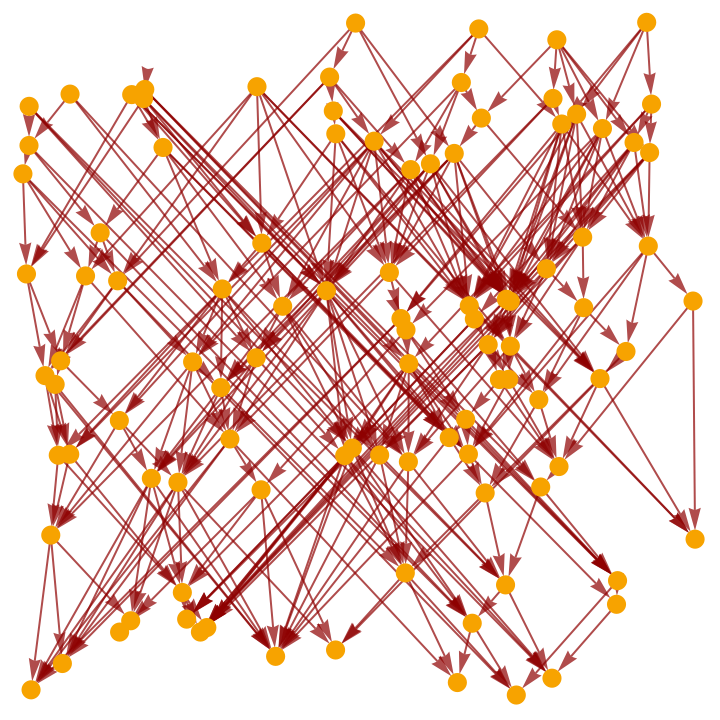
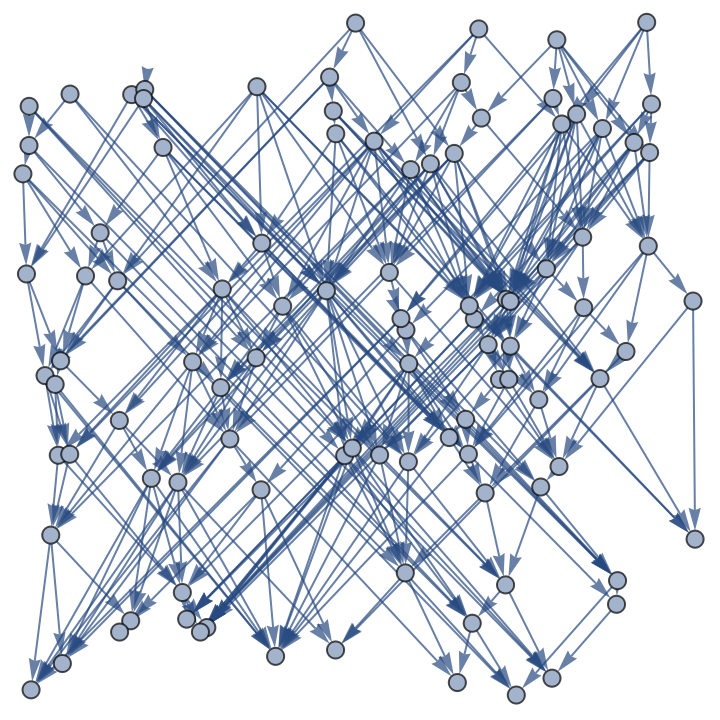
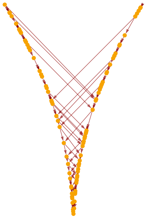
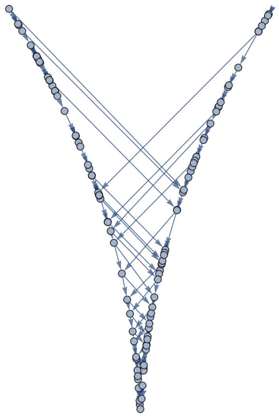
I used Wolfram Model’s “FlatSpacetimeSprinkling” [3] and “CurvedSpacetimeRegionSprinkling” [4] functions, to generate causal graphs for (1 + 1)D and (2+1)D flat Minkowski spacetime and (1 + 1)D and (2+1)D curved Schwarzschild spacetime. In the Schwarzschild metric case, corresponding to static black holes, the spacetime curvature is modeled according to Flamm’s paraboloid surface [6]. In the Kerr metric case, corresponding to rotating black holes, the surface is given by an integral equation [5], which makes implementation in the Sprinkling functions very complicated, and is therefore left as future work. The good thing is that the Kerr surface is closely related to Flamm’s paraboloid, so that one can grasp the main concept from the Schwarzschild case.
The number or density of the points in these discrete spaces can be dialed in the “Pre-Calculate Cases” section of the code using the parameter “numberevents”.
For each case, a causal graph is generated embedding causal paths as edges and, finally, event trajectories are calculated.
The results are displayed in the “Show Results” section.
Pre-calculate Cases
Pre-calculate Cases
In[]:=
numberevents=100;
1 + 1 D
1 + 1 D
In[]:=
cases={"1(+1)D-Flat","1(+1)D-Schwarzschild"};sprinkling=[2,numberevents],[4*Sqrt[Sqrt[x^2]]-y0,{x,y},{{-5,5},{0,5}},numberevents];coords=Map[#["PointsList"]&,sprinkling];causalgraph=Map[#["CausalGraph"]&,sprinkling];elist=Map[EdgeList[#]&,causalgraph];graph=MapThread[Graph[#1,#2,VertexCoordinates->#1]&,{coords,elist}];
Here we map the earliest and latest points.
In[]:=
earliest=Map[Position[Transpose[#][[2]],Max[Transpose[#][[2]]]][[1]][[1]]&,coords]latest=Map[Position[Transpose[#][[2]],Min[Transpose[#][[2]]]][[1]][[1]]&,coords];
Out[]=
{97,4}
In[]:=
MapThread[TableForm[{{#1,#2}}]&,{causalgraph,graph}]
Out[]=
,
2 + 1 D
2 + 1 D
In[]:=
cases2D={"2(+1)D-Flat","2(+1)D-Schwarzschild"};sprinkling2D=[3,numberevents],[4*Sqrt[Sqrt[x^2+y^2]]-z0,{x,y,z},{{-5,5},{-5,5},{0,6}},numberevents];surfplot={Plot3D[surf=0.5,{x,0,1},{y,0,1},PlotStyle->Directive[Opacity[0.05],Blue,Specularity[Black,10]],BoxedFalse,Axes->False,ColorFunctionScalingTrue,ColorFunctionFunction[{x,y,z},Hue[60-(z)^4]]],Plot3D[surf=4*Sqrt[Sqrt[x^2+y^2]],{x,-2.5,2.5},{y,-2.5,2.5},PlotStyle->Directive[Opacity[0.05],Blue,Specularity[Black,10]],BoxedFalse,Axes->False,ColorFunctionScalingTrue,ColorFunctionFunction[{x,y,z},Hue[60-(z)^4]],MeshFunctions->{#3&}]};coords2D=Map[#["PointsList"]&,sprinkling2D];causalgraph2D=Map[#["CausalGraph"]&,sprinkling2D];elist2D=Map[EdgeList[#]&,causalgraph2D];graph2D=MapThread[Graph[#1,#2,VertexCoordinates->#1]&,{coords2D,elist2D}];
In[]:=
surfplot
Out[]=
 ,

In[]:=
earliest2D=Map[Position[Transpose[#][[2]],Max[Transpose[#][[2]]]][[1]][[1]]&,coords2D]latest2D=Map[Position[Transpose[#][[2]],Min[Transpose[#][[2]]]][[1]][[1]]&,coords2D];
Out[]=
{55,25}
In[]:=
MapThread[TableForm[{{#1,#2}}]&,{causalgraph2D,graph2D}]
Out[]=
,
 |  |
 |  |
Show Results
Show Results
In[]:=
Manipulate[If[d==1,Manipulate[start=i;stop=k;sp=FindShortestPath[graph[[j]],coords[[j]][[start]],coords[[j]][[stop]]];spedge=Table[sp[[i]]sp[[i+1]],{i,1,Length[sp]-1}];Show[Graph[coords[[j]],spedge,VertexCoordinates->coords[[j]],EdgeStyle->{Blue,Opacity[0.9]}],AspectRatio->1,ImageSize->500,PlotLabel->cases[[j]]],{{j,2,"case"},1,Length[cases],1,AppearanceElements->All,Appearance"Open"},{{i,earliest[[2]]},1,Length[coords[[j]]],1,AppearanceElements->All,Appearance"Open"},{{k,latest[[2]]},1,Length[coords[[j]]],1,AppearanceElements->All,Appearance"Open"},SaveDefinitions->True],Manipulate[start=i;stop=k;sp2D=FindShortestPath[graph2D[[j]],coords2D[[j]][[start]],coords2D[[j]][[stop]]];spedge=Table[sp2D[[i]]sp2D[[i+1]],{i,1,Length[sp2D]-1}];Show[surfplot[[j]],Graph[coords2D[[j]],spedge,EdgeStyle->{Red,Opacity[1]},VertexCoordinates->coords2D[[j]],VertexSize.15*j^2/60*numberevents^(1.2)],AspectRatio->1,ImageSize->500,PlotLabel->cases2D[[j]],ViewPoint->Top],{{j,2,"case"},1,Length[cases2D],1,AppearanceElements->All,Appearance"Open"},{{i,earliest2D[[2]]},1,Length[coords2D[[j]]],1,AppearanceElements->All,Appearance"Open"},{{k,latest2D[[2]]},1,Length[coords2D[[j]]],1,AppearanceElements->All,Appearance"Open"},SaveDefinitions->True]],{{d,2,"dimensions"},1,2,1,Appearance"Open"},SaveDefinitions->True]
Out[]=


Conclusion
Conclusion
We can see that in the case of flat space, the resulting causal graph is isotropic. As a consequence, the trajectories are also isotropic and, sooner or later, each of the generated events in the space time will be reached by a trajectory. In the case of Schwarzschild’s curved spacetime, we see the events converging towards the singularity of the black hole. If the spacetime were continuous, the trajectory would eventually end up in the singularity. However, due to the discrete nature of the simulated spacetime, the trajectories might get trapped in quantum volumes that are at some distance from the singularity. In other words, in the quantum world it’s not possible to get down to infinitely small distances, and the trajectories of the events would never cross the singularity, but can get as close as to within a Planck’s length, ~1E(-33) cm. As stated earlier, this is a conclusion reached using the Schwarzschild curved spacetime. Most trajectories contemplate some anomalous jumps, which we could call “quantum leaps”, that are a consequence of the discretization of the spacetime. These are easier to see in the (1+1)D case, where the trajectory of the event suddenly jumps on the opposite branch of the surface. In a continuous spacetime these jumps would not happen as there would be a continuum of causal events next to the present one and on the same branch. Therefore these “quantum leaps” suggest a macroscopic signature of spacetime discretization. A logical, yet difficult next step for this project would be to formally integrate the Kerr integral equation into the Sprinkling functions, and visually represent this third case. However, given that Kerr’s surface is closely related to Flamm’s paraboloid, we can extend the observation to the rotating black hole case.
Keywords
Keywords
Flat Space Time
Curved Space Time
Black Hole
Schwarzchild Metric
Flamm’s Paraboloid
Kerr Metric
Discreteness
Curved Space Time
Black Hole
Schwarzchild Metric
Flamm’s Paraboloid
Kerr Metric
Discreteness
Acknowledgements
Acknowledgements
I would like to thank my mentor, William Munizzi, for his continual guidance and support throughout this project, Dr. Xerxes Ariswalla and Dr. Ahmed Elbanna for their indispensable help, and Dr. Stephen Wolfram and everyone at the Wolfram Fundamental Science Winter School for allowing me the opportunity to pursue such and exciting and relevant topic within the world of astrophysics .
References
References
[1] S. Wolfram, A New Kind of Science. (Wolfram Media, 2002).
[2] L. Smolin, Three Roads to Quantum Gravity. (Basic Books, 2017).
[3] J. Gorard, “FlatSpacetimeSprinkling,” Wolfram Function Repository, (Wolfram, 2020). (https://resources.wolframcloud.com/FunctionRepository/resources/FlatSpacetimeSprinkling/).
[4] J. Gorard, “CurvedSpacetimeRegionSprinkling,” Wolfram Function Repository, (Wolfram, 2020). (https://resources.wolframcloud.com/FunctionRepository/resources/CurvedSpacetimeRegionSprinkling/).
[5] R. Burghardt, “Drawing Kerr,” Journal of Modern Physics, 10(5), (2019).
[6] C. W. Misner, K. S. Thorne, J. A. Wheeler, Gravitation. (Princeton University Press, 2018).