This research explores the effect of varying levels of dropout regularization on neural networks through a practical application. More specifically, I focused on how different dropout rates can effect the accuracy of neural networks. Using a database containing the Electronic Health Records (EHRs) of thousands of diabetes patients collected from various healthcare providers, I created multiple networks with different dropout rates that were able to take in eight inputs and classify the data as either diabetes positive or diabetes negative. Before starting on the diabetes dataset, I proved the general concept using the Wolfram in-built Titanic Sample Data for which I created visualizations and a manipulation.
Introduction
Introduction
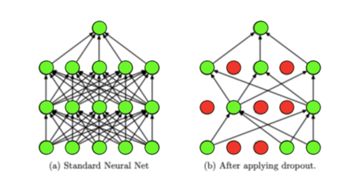
My project lies in the realm of machine learning, specifically within neural networks and dropout regularization. Machine learning is essentially using computer systems to process information and draw inferences or predictions from that data. These systems are able to learn and adapt without following explicit instructions.Within machine learning lies neural networks. Neural networks are computer systems modeled on the human brain. These systems have an input, multiple hidden layers, and an output. Within these hidden layers are multiple nodes, or artificial neurons, each connected to another and assigned a weight and threshold. If the output of any individual node is above the specified threshold value, that node is activated, sending data to the next layer of the network. Otherwise, no data from that neuron is passed to the next layer.Dropout regularization is a more advanced machine learning concept and is the focus of my project. Dropout regularization essentially "drops" random nodes at different points in time during training. This prevents overfitting (where the model fits the training data yet cannot accurately predict information based on new data) because the network does not fully rely on the training data as any node has the possibility of being killed. "Killing" a neuron is when the weight of the neuron is assigned to 0. This allows for networks to adapt to missing and incomplete information.Dropout regularization is implemented through integrating a dropout layer into the networks hidden layers which is assigned a specific dropout rate. A dropout rate (dRate) is the rate at which these nodes have the probability of dying. With a dropout rate of 0.2, for example, each node has a 20% chance of "dying off".Adapted from Srivastava, Nitish, et al. ”Dropout: a simple way to prevent neural networks from overfitting”, JMLR 2014
Proof of Concept
Proof of Concept
Data Collection and Organization
Data Collection and Organization
Before embarking on my project with a complex dataset, I wanted to see if the idea had any substance. I began to code a basic outline of what I wanted in my actual project just to visualize the general concept. My main goal with this was to discover how different dropout rates affects the distribution of outputs of various nets. I decided to use the classic "Titanic Survival" dataset which is in-built into Wolfram.
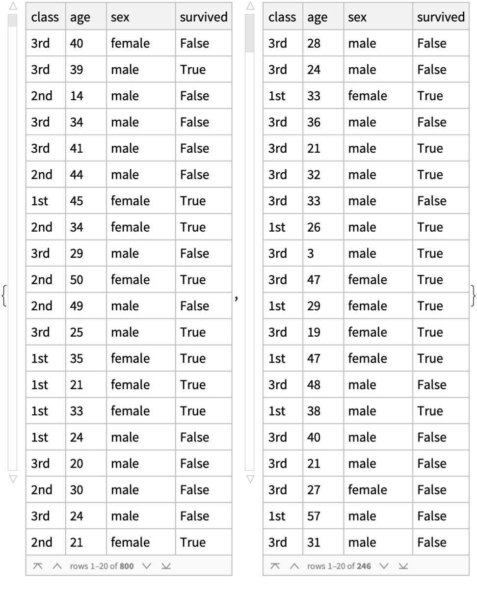
I began by calling the data from the Wolfram Data Repository and splitting it into a "training" and "testing" sample. The dataset contains the following information of titanic passengers:
◼
Economic Class (1st, 2nd, 3rd)
◼
Age
◼
Sex (Binary)
◼
Survived or Died (Binary)
Calling and organizing the data:
In[]:=
titanicData=;titanicData=DeleteMissing[titanicData,1,2];{trainData,testData}=TakeDrop[RandomSample@titanicData,800]
Out[]=
Neural networks cannot process strings, so the variables for "Class" and "Sex" need to be converted to a vector.
Converting the two variables to vectors:
In[]:=
classEncoder=NetEncoder[{"Class",{"1st","2nd","3rd"},"UnitVector"}]sexEncoder=NetEncoder[{"Class",{"male","female"},"UnitVector"}]
Out[]=
NetEncoder

Out[]=
NetEncoder
Constructing the Original Network Architecture
Constructing the Original Network Architecture
To create a neural net, the input, hidden layers, and output have to be specified. I outline the process of specifying this neural net with 3 inputs (class, age, sex) and 2 outputs (probability of survival, survival boolean). It is important to note that no dropout layers have been integrated yet.
Specifying neural network with dropout rate of 0:
In[]:=
netDataGraph=NetGraph[{CatenateLayer[]},{{NetPort["class"],NetPort["age"],NetPort["sex"]}->1},"class"->classEncoder,"age"->"Scalar","sex"->sexEncoder]
Out[]=
NetGraph

Initializing network:
In[]:=
netNormal=NetInitialize[NetGraph[{netDataGraph,LinearLayer[],LogisticSigmoid},{1->2->3->NetPort["survived"]},"survived"->"Boolean"]]
Out[]=
NetGraph
Training network:
In[]:=
trained0=NetTrain[netNormal,trainData,MaxTrainingRounds->1000]
Out[]=
NetGraph
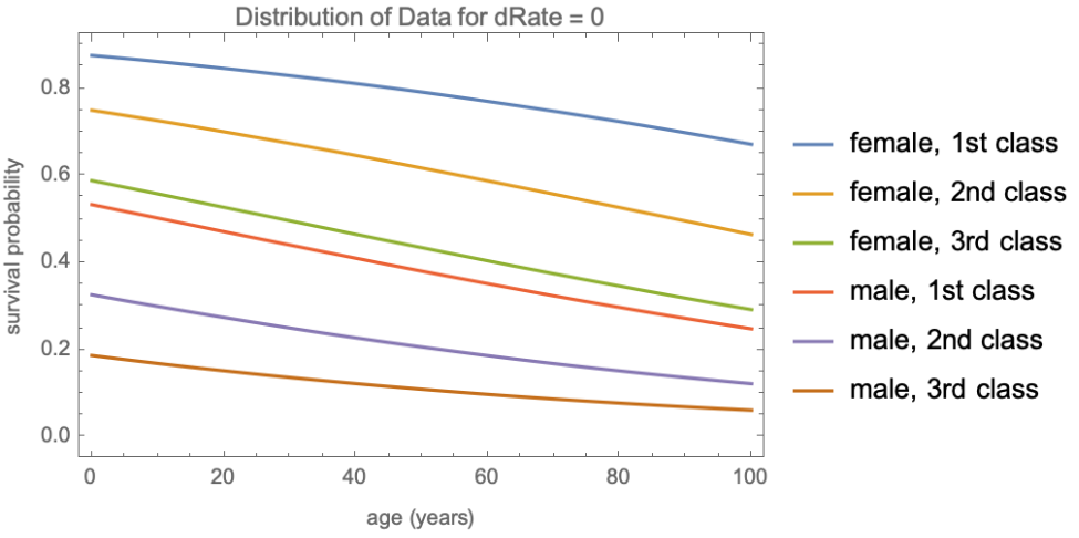
As my goal for this "Proof of Concept" was to see the effect of integrating higher dropout rates on the outputs of neural networks, I created a function which plots the distribution of outputs for a neural net.
Creates a function to plot the distribution of outputs for a dRate of 0:
In[]:=
plottingSurvival[class_,age_,sex_]:=trained0[<|"class"->class,"age"->age,"sex"->sex|>,None];plot0=Plot[{plottingSurvival["1st",x,"female"],plottingSurvival["2nd",x,"female"],plottingSurvival["3rd",x,"female"],plottingSurvival["1st",x,"male"],plottingSurvival["2nd",x,"male"],plottingSurvival["3rd",x,"male"]},{x,0,100},PlotLegends->{"female, 1st class","female, 2nd class","female, 3rd class","male, 1st class","male, 2nd class","male, 3rd class"},Frame->True,FrameLabel->{"age (years)","survival probability"},PlotLabel->"Distribution of Data for dRate = 0"]
Out[]=
Training Networks with Different Dropout Rates
Training Networks with Different Dropout Rates
dRate = 0.1
dRate = 0.1
Specifying neural network with dropout rate of 0.1:
Training neural network:
Plotting the distribution of outputs for a dRate of 0.1:
dRate= 0.2
dRate= 0.2
Initializing neural network with dropout rate of 0.2:
Training neural network with dropout rate of 0.2:
Plotting the distribution of outputs for a dRate of 0.2:
dRate = 0.3
dRate = 0.3
Initializing neural network with dropout rate of 0.3:
Training neural network:
Plotting the distribution of outputs for a dRate of 0.3:
dRate = 0.4
dRate = 0.4
Initializing neural network with dropout rate of 0.4
Training neural network:
Plotting the distribution of outputs for a dRate of 0.4:
dRate = 0.5
dRate = 0.5
Initializing neural network with dropout rate of 0.5:
Training neural network:
Plotting the distribution of outputs for a dRate of 0.5:
Calculating the Accuracy & Error
Calculating the Accuracy & Error
Since the dataset is quite small with a relatively low amount of inputs and outputs, I did not expect to see large changes in the accuracy and error of the neural nets with different dropout layers. In fact, because the data was so small, I predicted that turning off certain nodes would make the network less accurate due to a lack of processing power.
Putting all networks in a list to be called easier:
Finding the accuracy of each neural network:
Making the accuracy rates into coordinates:
Plotting the accuracy coordinates:
Finding the error of each neural network:
Making the error rates into coordinates:
Plotting the error coordinates:
Creating Manipulation
Creating Manipulation
The last task I wanted to perform with this dataset was to create a Manipulate which would allow users to find the probability of survival of a certain individual with the criteria of their choice. These inputs are:
◼
Class
◼
Sex
◼
Age
◼
Dropout Rate
The Manipulate would return, according to the specified dropout rate, a boolean (True or False) of whether the passenger would have survived, the probability of survival for that individual, as well as the plot for the specified dropout rate which shows the possible outputs for all other inputs.
Before working on the manipulate, I had to put all of the plots I created into a list and build a function that would process all of this data.
Before working on the manipulate, I had to put all of the plots I created into a list and build a function that would process all of this data.
Creating the list with all plots:
Building function:
Constructing the Manipulate:
Diabetes Dataset
Diabetes Dataset
Data Collection and Organization
Data Collection and Organization
Before beginning, I needed to collect the patient data and convert the strings into integers so that those list elements could be processed in the neural network. Here, I collect the dataset that contains the Electronic Health Records (EHRs) required for my network. The data contains an individual list for each patient which contains their :
◼
Gender
◼
Age
◼
Smoking History
◼
Body Mass Index (Measure of Body Fat Based on Height and Weight)
◼
Hemoglobin A1c Level (Average Blood Sugar Levels Over the Past 3 Months)
◼
Blood Glucose Level (Amount of Glucose in Bloodstream)
◼
Heart Disease - Binary
◼
Hypertension - Binary (High Blood Pressure)
◼
Diabetes - Binary
Collecting data from the Cloud:
Converting strings to integers:
In[]:=
Function to Re-Combine Data
Function to Re-Combine Data
Now that the strings can be converted to integers, I have to create a function that will replace the strings in the dataset to have lists containing numbers only and apply this function to all of the lists in the dataset.
Creating function:
Applying function to dataset:
In[]:=
Balancing the Modified Dataset
Balancing the Modified Dataset
I then needed to even out the "diabetes positive" and "diabetes negative" data to mitigate bias and ensure a balanced representation:
Plotting the original distribution of data:
Finding the amount of data by which to cut the larger dataset to:
Now, I can randomly "chop" the larger data portion to be equal to the "minimumElements" of the smaller dataset:
Plotting the new distribution of data:
In[]:=
Splitting Data
Splitting Data
After converting the list into integers and balancing the dataset, I can split the data into a training and testing set for the neural network to process.
Splitting data:
Constructing the Original Network Architecture
Constructing the Original Network Architecture
Before creating the neural network, I wanted to test whether the dataset was trainable in the first place. I performed a classification to determine this.
Using classification:
Since the "Accuracy" is a higher percentage than the "Accuracy Baseline", I know that the machine can learn from the data and predict more precisely than simply "guessing" the most frequent classification. These results serve as my confirmation to begin creating the network architecture for the diabetes dataset.
The architecture for the original network must specify the input, hidden layers, and output. It is important to note that there are no dropout layers integrated into the original neural net.
The architecture for the original network must specify the input, hidden layers, and output. It is important to note that there are no dropout layers integrated into the original neural net.
Constructing the layout of the original network:
Training Networks with Different Dropout Rates
Training Networks with Different Dropout Rates
Now that the original network with a dRate of 0 is created, I can essentially repeat this process with the implementation of 4 dropout layers, each with their designated dropout rate.
In[]:=
dRate = 0.1
dRate = 0.1
Creating the network:
Training the network:
dRate = 0.2
dRate = 0.2
Creating the network:
Training the network:
dRate = 0.3
dRate = 0.3
Creating the network:
Training the network:
dRate = 0.4
dRate = 0.4
Creating the network:
Training the network:
dRate = 0.5
dRate = 0.5
Creating the network:
Training the network:
dRate = 0.6
dRate = 0.6
Creating the network:
Training the network:
dRate = 0.7
dRate = 0.7
Creating the network:
Training the network:
dRate = 0.8
dRate = 0.8
Creating the network:
Training the network:
dRate = 0.9
dRate = 0.9
Creating the network:
Training the network:
Calculating the Accuracy & Error
Calculating the Accuracy & Error
After training all of the networks, I wanted to discover the most accurate network in predicting diabetes in patients. To do so, I have to create a list that includes all of the trained neural networks that have the varying dropout rates. This will save me from having to call every single net in the future as I can simply call the index of the list. After that, I have to determine the accuracy of each network. There are two ways of doing so. I will outline both.
Creating the list of all of the trained neural networks:
NetMeasurements
NetMeasurements
First, I can determine the accuracy of the networks using Wolfram's in-built NetMeasurements function. I can also use NetMeasurements to determine the error rate of each network.
Calculating the accuracy rates:
Making the rates into coordinates:
Plotting the accuracy rates:
Calculating the error rates:
Making the rates into coordinates:
Plotting the error rates:
Precision & Recall
Precision & Recall
In the precision and recall method, I have to use different equations to determine the accuracy of the neural network. First, I have to find the "True Positives", "True Negatives", "False Positives", and "False Negatives". This is done by creating the list of all of the actual diagnoses in the testing data then cross referencing those with the diagnoses created by each individual neural net.
Finding the diagnoses of the testing data:
Creating lists of the outputs of the neural networks for each data list:
Creating Function
Creating Function
Now I will create the function that will determine the "True Positive", "True Negative", "False Positive", and "False Negative" values for each neural network in relation to the actual values.
Creating function:
Calculating Precision: TP/(TP + FP)
Calculating Precision: TP/(TP + FP)
Precision rates can be calculated by dividing the amount of "True Positives" by the sum of the "True Positives" and "False Positives". This formula was abstracted from the Google developers page on Machine Learning.
Creating a list with all precision values:
Making those values into coordinates:
Plotting the coordinates:
Recall = TP/(TP + FN)
Recall = TP/(TP + FN)
Recall rates can be calculated by dividing the amount of "True Positives" by the sum of the "True Positives" and "False Negatives" . This formula was abstracted from the Google developers page on Machine Learning .
Creating a list with all recall values:
Making those values into coordinates:
Plotting the coordinates:
Conclusion
Conclusion
Overall, I was able to conclude that a dRate of 0.2-0.3 is ideal for the diabetes dataset. Similar to this practical application in medicine, even 0.5-1 percent more accurate predictions can be very important. It is possible that the optimal dropout rate is low because of the simplicity of the data. With images, the best rate would most likely be higher as the network architecture would be more complex as well.
Future Work
Future Work
In this research program, I essentially had to learn machine learning from the ground up. Therefore, I spent a considerable amount of time performing in-depth research and essentially "absorbing" information about neural networks. In the future, it would be cool to see the implementation of larger data sets and possibly even image classification. I initially tried to use a dataset of MRI images in the attempt of classifying tumors with my neural network, yet we learned (the hard way) that my computed did not have the power to process that. Being able to achieve above a 90% accuracy on a diabetes dataset shows how the possibilities are endless.
References
References
◼
“Building and Training Basic Neural Networks.” Wolfram Videos: Building and Training Basic Neural Networks, www.wolfram.com/broadcast/video.php?c=105&disp=list&v=1838. Accessed 13 July 2023.
◼
CampusX. “Dropout Layer in Deep Learning | Dropouts in Ann | End to End Deep Learning.” YouTube, 12 May 2022, www.youtube.com/watch?v=gyTlcHVeBjM.
◼
“Classification: Precision and Recall | Machine Learning | Google for Developers.” Google, developers.google.com/machine-learning/crash-course/classification/precision-and-recall. Accessed 13 July 2023.
◼
McNealis, Nisha. “A Simple Introduction to Dropout Regularization (with Code!).” Medium, 30 Apr. 2020, medium.com/analytics-vidhya/a-simple-introduction-to-dropout-regularization-with-code-5279489dda1e.
◼
Mustafa, Mohammed. “Diabetes Prediction Dataset.” Kaggle, 8 Apr. 2023, www.kaggle.com/datasets/iammustafatz/diabetes-prediction-dataset.
◼
Sanagapati, Pavan. “What Is Dropout Regularization? Find Out :).” Kaggle, 21 July 2019, www.kaggle.com/code/pavansanagapati/what-is-dropout-regularization-find-out/notebook.
◼
Acknowledgements
Acknowledgements
◼
Nicolò Monti - Thank you for being an amazing teacher, I could not have done this without you.
◼
Karan Chakravarthy - Thank you for all of your help with my challenges and leading me to the solution
◼
Athanasios Paraskevopoulos - Thank you for being an awesome mentor and helping me when I needed it.
◼
All of the Teaching Assistants & Directors at the Research Program
CITE THIS NOTEBOOK
CITE THIS NOTEBOOK
Enhancing diabetes prediction through the optimization of dropout regularization
by Kartik Mathur
Wolfram Community, STAFF PICKS, July 13, 2023
https://community.wolfram.com/groups/-/m/t/2964575
by Kartik Mathur
Wolfram Community, STAFF PICKS, July 13, 2023
https://community.wolfram.com/groups/-/m/t/2964575