This notebook assembles a compact toolkit for finite-dimensional quantum information. It defines computational and operator bases, establishes Hilbert–Schmidt orthonormality, and shows how quantum objects transform under unitary change of basis. It explains vectorization with Kronecker products and clarifies the relation between matrices and states. It formalizes bipartitions of a Hilbert space, constructs product and local bases, reshapes state vectors into coefficient matrices, and applies local unitaries. It then connects the singular value decomposition to the Schmidt decomposition of pure bipartite states, linking singular values to spectra of reduced density matrices and standard entanglement measures, including von Neumann and Rényi entropies. Throughout, it includes checks for orthonormality, unitarity, and spectrum preservation, offering practical patterns for entanglement analysis and tensor-product manipulations.
Note: Most equality checks should return True. However, rerunning code may produce False due to machine precision numerical errors. In such cases, use lhs - rhs // Chop instead of lhs == rhs to verify that only zero terms remain.
Vector and operator bases
Vector and operator bases
We work in a finite-dimensional complex Hilbert space of dimension .
d
In[]:=
d=3;
Define a generic complex-valued square matrix in above dimension:
In[]:=
mat=RandomComplex[{-1-I,1+I},{d,d}];mat//MatrixForm
Out[]//MatrixForm=
-0.691204+0.735668 | -0.790681+0.723384 | -0.347047-0.260592 |
0.733252-0.210214 | -0.362732+0.496197 | -0.252181-0.278482 |
-0.698769-0.389951 | 0.33211+0.81806 | -0.990198+0.573962 |
For the dimension , pick three independent 3D-vectors
d=3
In[]:=
basis=Table[UnitVector[d,j],{j,d}]
Out[]=
{{1,0,0},{0,1,0},{0,0,1}}
The above basis (the set of unit vectors i.e., the rows/columns of the identity matrix) is usually called the computational basis. It is in fact a vector basis. In quantum literature, each of above vectors is usually represented by a ket, usually indexed as , , …, .
|0〉
|1〉
|d-1〉
The computational basis equals the set of rows (or columns) of the identity matrix:
In[]:=
basis==IdentityMatrix[d]
Out[]=
True
Elements of the computational basis are orthonormal :
〈i|j〉=
δ
i,j
In[]:=
OrthogonalMatrixQ[basis]
Out[]=
True
A different way of checking above vectors are explicitly orthogonal ():
=.=
v
i
v
j
†
v
i
v
j
δ
i,j
In[]:=
ConjugateTranspose[basis].basis//Chop//MatrixForm
Out[]//MatrixForm=
1 | 0 | 0 |
0 | 1 | 0 |
0 | 0 | 1 |
From a vector basis we obtain a canonical operator basis (i.e. a basis for operators in the Hilbert space). The canonical choice is the set of matrix units. This can be done using the Kronecker product ):
⊗
v
i
†
v
j
Out[]=

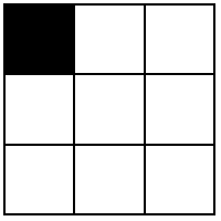
Note the complex conjugation. Although it is not crucial here, basis vectors may be complex in general. In these examples, conjugation suffices; you need not take a conjugate transpose; see the below example.
†
{,,…,}
a
1
a
2
a
n
b
1
b
2
b
n
*
{,,…,}
a
1
a
2
a
n
b
1
b
2
b
n
In[]:=
Modulea=Arraya.,{3},b=Arrayb.,{3},ConjugateTranspose[a].b==Conjugate[a].b
Out[]=
True
The operator basis introduced above satisfies the Hilbert-Schmidt orthonormality relation
Tr.=
†
E
i,j
E
k,l
δ
i,k
δ
j,l
In[]:=
Outer[Tr[ConjugateTranspose[#1].#2]&,matBasis,matBasis,2]==Table[KroneckerDelta[i,k]KroneckerDelta[j,l],{i,d},{j,d},{k,d},{l,d}]
Out[]=
True
Any operator can be expanded uniquely as
M=|i〉〈j|=
∑
i,j
M
i,j
∑
i,j
M
i,j
E
i,j
In[]:=
ArrayDot[mat,matBasis,2]==mat
Out[]=
True
Of course, the above choice of basis for a give dimension is not the only way to find orthonormal basis. There are infinitely many ways to do so. Let’s find a new complex orthonormal basis:
In[]:=
newBasis=Orthogonalize@RandomComplex[{-1-I,1+I},{3,3}]
Out[]=
{{-0.486145-0.556007,-0.476115+0.14332,0.368199+0.267809},{-0.0204355-0.042848,-0.189957-0.634514,0.378622-0.644748},{0.182362-0.647309,0.397974+0.394586,-0.024548-0.482752}}
By construction, we take the basis vectors to be orthonormal. Although a non-orthonormal basis may be chosen, it can always be converted into an orthonormal one. For simplicity, we assume an orthonormal basis throughout, applying a procedure such as the Gram–Schmidt algorithm (see Orthogonalize documentation) if necessary.
Check the basis elements are orthonormal
In[]:=
ConjugateTranspose[newBasis].newBasis//Chop//MatrixForm
Out[]//MatrixForm=
1. | 0 | 0 |
0 | 1. | 0 |
0 | 0 | 1. |
Let and be orthonormal bases. The change‑of‑basis unitary is =. A matrix represented in the basis is mapped to the basis as .
{|〉}
v
i
{|〉}
w
i
U
ij
v
i
w
j
M
{|〉}
w
i
{|〉}
v
i
M'=U.M.
†
U
Define a unitary transformation that we use to transform a matrix from one basis to another one:
In[]:=
u=Outer[Conjugate[#1].#2&,newBasis,basis,1];u//MatrixForm
Out[]//MatrixForm=
-0.486145+0.556007 | -0.476115-0.14332 | 0.368199-0.267809 |
-0.0204355+0.042848 | -0.189957+0.634514 | 0.378622+0.644748 |
0.182362+0.647309 | 0.397974-0.394586 | -0.024548+0.482752 |
The above computation can be written as in Dirac notations: with and are two orthonormal bases
u=|〉
∑
i,j
v
i
w
j
v
i
w
j
Check it is unitary:
In[]:=
UnitaryMatrixQ[u]
Out[]=
True
Matrix transformation into new basis:
m'=u.m.
†
u
In[]:=
matInNewBasis=u.mat.ConjugateTranspose[u];matInNewBasis//MatrixForm
Out[]//MatrixForm=
-0.243842+1.50141 | -0.16306-0.0644583 | 0.198234+0.216222 |
0.194143-0.412039 | -0.320471+0.516205 | -0.666171+0.0526952 |
0.0481686+0.0298917 | -0.42789+0.558243 | -1.47982-0.211788 |
Calculate 〈|m|〉 (or can be written as .m.⊗) and show it is the same as the matrix representation in the new basis
∑
i,j
w
i
w
j
w
i
w
j
∑
i,j
*
w
i
w
j
w
i
*
w
j
In[]:=
Outer[Conjugate[#1].mat.#2&,newBasis,newBasis,1]==matInNewBasis//Chop
Out[]=
True
Alternatively, one may perform basis transformations via vectorization, where the columns of a matrix are stacked sequentially to form a single vector: .
vec[U.M.]=(⊗U).vec[M]
†
U
*
U
Define a function for vectorization:
In[]:=
ClearAll[vectorize]vectorize[m_]:=Flatten[Transpose@m]
Show one example for a 3x3 matrix
In[]:=
MatrixFormArraya.,{3,3}->MatrixFormvectorizeArraya.,{3,3}
Out[]=
a.[1,1] | a.[1,2] | a.[1,3] |
a.[2,1] | a.[2,2] | a.[2,3] |
a.[3,1] | a.[3,2] | a.[3,3] |
a.[1,1] |
a.[2,1] |
a.[3,1] |
a.[1,2] |
a.[2,2] |
a.[3,2] |
a.[1,3] |
a.[2,3] |
a.[3,3] |
One can also define a function for reversing the above process (here we consider unvectorize for only square matrices):
Unvectorize reverses vectorize:
In[]:=
unvectorize[m_]:=Transpose@Partition[m,Sqrt@Length@m]
Check that unvectorize reverse vectorize operation :
unvec[vec[M]]=M
In[]:=
Witha=Arraya.,{3,3},unvectorize@vectorize[a]==a
Out[]=
True
Check which is the same as
(⊗u).vec[m]=vec[m']
*
u
unvec[(⊗u).vec[m]]=m'
*
u
In[]:=
KroneckerProduct[Conjugate[u],u].vectorize[mat]==vectorize@matInNewBasisunvectorize[KroneckerProduct[Conjugate[u],u].vectorize[mat]]==matInNewBasis
Out[]=
True
Out[]=
True
Using above basis, let’s find a basis for matrices (i.e. a basis for operators in the Hilbert space). The canonical choice is the set of matrix units. This can be done using the Kronecker product ):
⊗
v
i
†
v
j
Bipartitions
Bipartitions
Set the dimension of the Hilbert space:
Find the dimension’s prime factorization:
Multiplying across the new list yields the original number:
Let us partition the factors into two ordered subsets. The complete set of possible combinations is given as follows.
For each possible combination, determine the overall dimensionality of each subset.
Fix a bipartition:
Choose orthonormal bases:
Define corresponding unitaries that transforms computational basis from each subspace into above bases (note that the columns of each unitary are the corresponding bases):
Check both are unitary:
Composite system has the product basis:
Represent the basis using its indices:
Take home lessons
Take home lessons
Bipartitions and the Schmidt decomposition
Bipartitions and the Schmidt decomposition
We shall work only in the computational bases from this point on.
Product state (separable case)
Product state (separable case)
Let’s create a separable state randomly:
Take the singular value decomposition (SVD) of the state:
Pay attention to the corresponding dimensions:
Sine σ is a diagonal matrix, take its diagonal elements:
Create list of all terms in the Schmidt basis:
As mentioned, only one term from Schmidt basis has nonzero coefficient because the original state was separable.
Of course, as expected, the above state is the same as the original one:
Generate all elements of Schmidt basis:
Find representation of the state in the Schmidt basis:
Of course, as expected only one term is nonzero and that coefficient is the same as the singular value of state
Entangled case (non-separable)
Entangled case (non-separable)
Obviously, if the state is not separable, more than one singular values would be nonzero.
Create a pure state directly in the bipartitioned dimension in the computational basis:
Find the corresponding nonzero singular values (they are also called Schmidt coefficients):
Since there are more than one Schmidt coefficients, it means that the state is not separable (i.e. it is entangled) and cannot be written as a product of subsystem states.
Find the SVD of the state:
Diagonal elements of σ are singular values
Define two local unitaries:
Check local unitary invariance:
Spectral match: reduced density matrices have the same nonzero eigenvalues
Show that the eigenvalues of reduced density matrices are the same as square of the singular values:
Wolfram quantum framework
Wolfram quantum framework
The analysis above was intended as a pedagogical exploration of the applications of Singular Value Decomposition (SVD) in quantum information and science. It is important to note that these techniques and tools are seamlessly integrated within the Wolfram Quantum Framework. In what follows, I will briefly review how this integration is realized.
Install Wolfram Quantum Framework:
Quantum objects include a summary box with key information (expandable via the plus sign) and can also be displayed in standard forms such as Dirac notation.
Return the state in the Dirac notation:
For bipartition, treat it as a state property given as a string, with the second argument specifying the first subsystem’s dimension.
Divide the Hilbert space into two subsystem with the first subsystem having the dimension 3
If you do not give any dimension, we will get the divisor of the overall dimension and set the dimension of first subsystem as the largest integers that divides the dimension.
Give no dimension for the first subsystem, and we set it as 5 automatically
Pay attention to minor difference in dimensions:
Schmidt decomposition does not require bipartition first; the “SchmidtBasis” property accepts the first subsystem’s dimension as an argument.
Display the state after Schmidt decomposition in Dirac notation:
Show nonzero terms in above linear combination (Schmidt coefficients):
Show they are the same as the singular values we obtained before (of course, trivial result):
CITE THIS NOTEBOOK
CITE THIS NOTEBOOK
Bipartitions and the SVD-Schmidt: A quantum information toolkit
by Mohammad Bahrami
Wolfram Community, STAFF PICKS, August 28, 2025
https://community.wolfram.com/groups/-/m/t/3536668
by Mohammad Bahrami
Wolfram Community, STAFF PICKS, August 28, 2025
https://community.wolfram.com/groups/-/m/t/3536668