ORIGINAL DEMONSTRATIONS: Klaus von Bloh,
“Causal Interpretation of the Free Quantum Particle”,
“Causal Interpretation of the Double-Slit Experiment in Quantum Theory”,
“Triple-Slit Experiment in the Causal Interpretation”,
“Bohm Trajectories for Quantum Particles in a Time-Dependent Linear Potential”,
“Causal Interpretation for an Electron Passing through Two Narrow Slits”,
“Continuous Transition between Classical and Bohm Quantum Pictures for Young's Interference Experiment”,
Wolfram Demonstrations Project. DOI: http://dx.doi.org/10.13140/RG.2.2.13161.06242
Abstract: The causal interpretation of Quantum Theory, often called “Bohmian Mechanics” or “Non-local Hidden Variable Theory”, also known as the de Broglie-Bohm interpretation, is a unique and deterministic approach to understanding quantum mechanics. Bohmian mechanics draws inspiration from Louis de Broglie’s 1923 proposition of the “double solution.” Independently of de Broglie, David Bohm developed his theory in 1952. This interpretation provides an alternative perspective on the fundamental nature of non-relativistic quantum phenomena. In the causal Interpretation, particles are described not only by complex valued wavefunction in the Hilbert space but also by real positions that evolve deterministically in time, guided by a “quantum potential” or by the gradient of the phase function derived from the wavefunction. The theory offers a coherent account of quantum phenomena, reconciling the probabilistic behavior of particles with a deterministic underlying dynamics.This notebook provides a concise overview of the main principles of Bohmian mechanics by applying Fourier analysis to one - dimensional simple problems. Furthermore the concept of pilot waves and the role of the quantum potential in influencing particle trajectories are investigated. Another important aspect is the non-local nature of Bohmian mechanics, where particles can be correlated across spatially separated regions, connected with each other superluminally, but this will not be discussed here. But anyway, the causal interpretation gives a deeper insight into the behavior of particles at the quantum level and their unique properties in wave-particle duality.
Introduction
Introduction
In 1952, David Bohm’s intention in proposing an alternative formulation of quantum mechanics was to address some of the foundational issues and paradoxes that were inherent in the standard interpretation of quantum theory[1,2,13,14]. He aimed to provide a more causal and intuitive description of quantum phenomena by introducing hidden variables and the concept of a pilot wave, without extensively exploring the specific origin of the pilot wave. Bohm’s motivation was to find a way to reconcile the probabilistic nature of quantum mechanics with a more classical understanding of the behavior of particles, ultimately aiming to provide a deeper and clearer understanding of the underlying reality of quantum systems. His intention was not to revert to classical mechanics, but rather to elucidate aspects such as the non-locality inherent in the quantum theory.
The name hidden variable theory arises from the assumption that the wavefunction does not provide a complete description of a quantum mechanical system, and that there are additional hidden variables that could potentially make the wavefunction a deterministic, objective foundation or property for single particles.These hidden variables are considered to supplement the wavefunction with additional information, but they are not directly observable. In this non-local hidden variable theory, it is more accurate to say that the initial positions of particles are hidden and not experimentally determinable. Ironically, the common statement is often made that the positions of particles, in general, are hidden and only become definite through measurement. In reality, a more precise statement would be that the wavefunction itself is hidden. In 1926 Erwin Madelung, a German physicist, made a first significant contribution to the “Bohmian view” by developing an alternative representation where the Schrödinger equation is transformed into a continuity equation. His formulation inadvertently introduced key elements that later became essential to the development of Bohmian mechanics.
The name hidden variable theory arises from the assumption that the wavefunction does not provide a complete description of a quantum mechanical system, and that there are additional hidden variables that could potentially make the wavefunction a deterministic, objective foundation or property for single particles.These hidden variables are considered to supplement the wavefunction with additional information, but they are not directly observable. In this non-local hidden variable theory, it is more accurate to say that the initial positions of particles are hidden and not experimentally determinable. Ironically, the common statement is often made that the positions of particles, in general, are hidden and only become definite through measurement. In reality, a more precise statement would be that the wavefunction itself is hidden. In 1926 Erwin Madelung, a German physicist, made a first significant contribution to the “Bohmian view” by developing an alternative representation where the Schrödinger equation is transformed into a continuity equation. His formulation inadvertently introduced key elements that later became essential to the development of Bohmian mechanics.
Use the following command, if you need to save/export graphs created by Mathematica into the current notebook directory:
In[]:=
SetDirectory[NotebookDirectory[]]
Out[]=
I:\KlausMemory
Feel free to use, reproduce, and modify this code in its entirety or in part of it .
To make the equations more readable, the standard form of partial derivatives is used. The definition is taken from the Wolfram blog.
In[]:=
pdConv[f_]:=TraditionalForm[f/.Derivative[inds__][g_][vars__]:>Apply[Defer[D[g[vars],##]]&,Transpose[{{vars},{inds}}]/.{{var_,0}:>Sequence[],{var_,1}:>{var}}]]
A further note : Some descriptions might be formulated too simply and could possibly require a more detailed explanation.
The Schrodinger Equation
The Schrodinger Equation
The motion of particles obeying the Schrödinger equation for a system of particles is defined in a -dimensional configuration space, where each particle’s position is represented by three coordinates (). The Schrödinger equation was formulated by Erwin Schrödinger in 1926. The equation is a partial differential equation that represents the time evolution of the wavefunction of a quantum system. The wavefunction, denoted by , where is an element of the Hilbert space, contains all the information about the quantum system, including the probabilities of different outcomes of measurements. The Schrödinger equation shows how the wavefunction changes with time and is given by
N
3N
x,y,z
Ψ
Ψ
iħ ∂Ψ/∂t = HΨ
where is the imaginary unit, is the reduced Planck' s constant, t represents time, is the partial derivative with respect to time, is the wavefunction, and H is the Hamiltonian operator, representing the total energy of the system. The Hamiltonian operator is defined as the sum of the kinetic energy and the potential energy operators. The Hamiltonian operator is a Hermitian operator, meaning that its adjoint is equal to itself. For a single particle, it is given by:
i
ħ
∂/∂t
Ψ
H
H=T+V
where T is the kinetic energy operator, representing the energy associated with the particle' s motion, and V is the potential energy operator, representing the energy associated with the particle' s interaction within the system. Solving the Schrödinger equation with the Hamiltonian operator allows us to determine the energy levels and corresponding wavefunctions for a given potential.
The Current Density and the Velocity of a Single Particle
The Current Density and the Velocity of a Single Particle
In classical physics the current density is a vector field that represents the flow of density or charge density. It describes the rate at which density is flowing in a particular direction at each point in space. Mathematically, the current density is denoted by the symbol “j” and is given by: =ρ
j
j
v
ρ is the density, representing the squared modulus of the wavefunction (=Ψ). is the velocity vector of the particle, .
2
(|Ψ|)
*
Ψ
v
The current density plays a crucial role in Bohmian mechanics as it is related to the continuity equation, which ensures the conservation of density [12]. It provides insights into the flow of density in quantum systems and is fundamental to understanding the behavior of particles at the quantum level.
j
From the continuity equation, it follows that the gradient (here, one-dimensional) of the phase function of the wavefunction ( eikonal form: ) gives the particle’s momentum =m=S. Immediately, it follows from the momentum for the velocity field of a single particle=S,where is the mass of the particle. The initial position of a single particle is fixed by the initial probability density and could not be arbitrarily chosen. Here, in one-dimension: means .
Ψ
Ψ=R*
/ℏS
e
p
v
∇
v
∇
m
m
∇
∂
∂x
In the Bohmian interpretation, the normalization factor and the reduced Planck’s constant have no influence on the velocity field, as it cancels out in the equations.
ℏ
To get the gradient of the phase function which correspondent to the velocity the wavefunction must be defined in the eikonal form (see the next chapter).
Ψ
*
Ψ
In[]:=
Psi[x_,t_]=R[x,t]ExpS[x,t];PsiC[x_,t_]=Psi[x,t]/.Complex[0,n_]->-Complex[0,n](*complexconjugate*);Print["Velocity: "]vx[x_,t_]=(D[Psi[x,t],x]/Psi[x,t]-D[PsiC[x,t],x]/PsiC[x,t])//Simplify//pdConv
ℏ
*
Ψ
-Iℏ
2m
Velocity:
Out[]//TraditionalForm=
∂S(x,t)
∂x
m
or in short
In[]:=
vx[x_,t_]=SimplifyImPsi[x,t]//ComplexExpand,AssumptionsElement[_,Reals]
ℏ
m
∂
x
Psi[x,t]
Out[]=
(1,0)
S
m
The Wavefunction Ψand the Hamilton Jacobi Formulation of the Schrodinger equation
The Wavefunction and the Hamilton Jacobi Formulation of the Schrodinger equation
Ψ
The eikonal form or often called polar form of the wavefunction is represented as , where is the amplitude or magnitude of the wavefunction or better called amplitude of the field, and S is the phase function. From here on, the eikonal form of the wavefunction will be referred to as the “polar form.” The amplitude of the wavefunction indicates the strength of the waves or field, while the phase describes the position and relative velocity of the particle. Together, amplitude and phase determine the motion of quantum objects in wave mechanics. The analogy originates from classical wave mechanics. In orthodox quantum theory, the square of the amplitude (|=ρ=) gives the probabiity density distribution of finding the particle (it is not the density of the particle itself). The particle motion is guided by the gradient of the phase function from the wavefunction. The significance of the phase lies in its description of the relative displacement of the particle at different points in space. To emphasize the significance of the Bohmian interpretation, the probability function is consistently referred to as the density function (of the field).
Ψ=R*expS
i
ħ
R
Ψ
R
R
2
(|Ψ|)
2
R
S
ψ
Figure
0
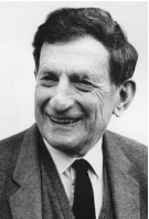
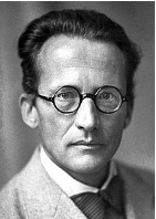
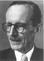
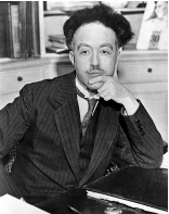
. David Bohm, Erwin Schrödinger, Erwin Madelung and Louis de Broglie (images from [Wikipedia and Alchetron]). For the one - dimensional case, the Schrödinger equation is given by
In[]:=
SE[u_]:=u+V[x]u-ℏuSEC[u_]:=u+V[x]u+ℏu
-
2
ℏ
2m
∂
{x,2}
∂
t
-
2
ℏ
2m
∂
{x,2}
∂
t
i
i=
(-1)
ħ
t
m
x
V(x)
In quantum mechanics, the modified Hamilton-Jacobi equation is a system of two partial differential equation that provides an alternative representation of the Schrödinger equation. The modified Hamilton-Jacobi equation is an eikonal like equation, representing a particular type of wavefunction known as the “action-phase wavefunction” or “eikonal function.” The solution to the Hamilton-Jacobi equation provides information about quantum mechanics in a formalism closer to classical concepts, such as Hamiltonian mechanics. To get the modified Hamilton Jacobi equations the wavefunction must be defined in the polar form[1,11].
In[]:=
Psi[x_,t_]=R[x,t]ExpS[x,t]PsiC[x_,t_]=Psi[x,t]/.Complex[0,n_]->-Complex[0,n](*complexconjugate*)eq1=SE[Psi[x,t]]0;eq2=SEC[PsiC[x,t]]0;Solve{eq1,eq2},[x,t],[x,t]//Simplify//Expand//Flatten//pdConv
ℏ
*
Ψ
(0,1)
S
(0,1)
R
Out[]=
S[x,t]
ℏ
Out[]=
-
S[x,t]
ℏ
Out[]//TraditionalForm=
R(x,t)--V(x),--
∂S(x,t)
∂t
2
ℏ
2
∂
∂
2
x
2mR(x,t)
2
∂S(x,t)
∂x
2m
∂R(x,t)
∂t
R(x,t)S(x,t)
2
∂
∂
2
x
2m
∂R(x,t)
∂x
∂S(x,t)
∂x
m
From the first equation the term (one-dimensional) or (multi-dimensional with the Laplace-Operator ) is called quantum potential, which introduces an additional term to the classical Hamilton-Jacobi equation. From the second equation the continuity equation ρ+j=0 with the current (=velocity, =wave density) can be derived by applying the squared quantum amplitude . In this case, an alternative representation of the wavefunction could be formulated by setting: with the wave density .
-R(x,t)
2
ℏ
2m
1
R(x,t)
2
∂
∂
2
x
-R(,t)
2
ℏ
2m
2
∇
r
R(t)
r,
2
∇
∂
∂t
∂
∂x
j=ρv
v
ρ
2
R
R(x,t)=
ρ(x,t)
ρ
In[]:=
Psi[x_,t_]=S[x,t]PsiC[x_,t_]=Psi[x,t]/.Complex[0,n_]->-Complex[0,n]eq1=SE[Psi[x,t]]0;eq2=SEC[PsiC[x,t]]0;solve=Solve{eq1,eq2},[x,t],[x,t]//FullSimplify//Expand//Flatten//pdConv
ρ[x,t]
Exp
ℏ
(0,1)
S
(0,1)
ρ
Out[]=
S[x,t]
ℏ
ρ[x,t]
Out[]=
-
S[x,t]
ℏ
ρ[x,t]
The Quantum Potential
The Quantum Potential
In the three (or multi) - dimensional case:
The Superposition Rule für Wavefunction in the Polar Form
The Superposition Rule für Wavefunction in the Polar Form
The rule for the superposition of wavefunctions in the polar form is [11]:
The Position Space and Momentum Space in Quantum Mechanics
The Position Space and Momentum Space in Quantum Mechanics
The Fourier Solution of a Free Particle in the One-dimensional Case
The Fourier Solution of a Free Particle in the One-dimensional Case
The Quantum Amplitude, the Phase Function, the Velocity and the Quantum Potential
The Quantum Amplitude, the Phase Function, the Velocity and the Quantum Potential
To obtain the quantum amplitude and the phase function, the following transformations need to be performed.
The normalization factor, which is not important for the motion, could be calculated by
Proof the correctness
The integration with respect to time leads to the following analytical solutions.
Expectation Values
Expectation Values
1.) Position Expectation Value : This represents the average position of a particle in a given state, expressed by the normalized density.
2.) Momentum Expectation Value : This gives the average momentum of a particle in a given state, expressed by the normalized density. .
3.) Kinetic Energy Expectation Value: This gives the average kinetic energy of a particle in a given state, expressed by the normalized density and the Hamilton operator.
Snapshots
Snapshots
To observe how everything interacts, the density, the velocity field and the quantum potential are displayed together.
The Motion in an Uniform Field
The Motion in an Uniform Field
Using the following ansatz
The above ordinary differential equation (ODE) is satisfied with the following ansatz .
Transformation into the positions-space leads to the unnormalized wavefunction.
The Quantum Amplitude, the Phase Function, the Velocity and the Quantum Potential
The Quantum Amplitude, the Phase Function, the Velocity and the Quantum Potential
The normalization factor, which is not important for the motion, could be calculated by
Proof the correctness
To check the continuity equation
The integration with respect to time leads to the following analytical solutions.
Snapshots
Snapshots
To observe how everything interacts, the density, the velocity field and the quantum potential are displayed together. On the youTube channel you can see an animation [14].
To complete the information about the wavefunction, the normalized wavefunction with all parameter will be given:
Expectation Values
Expectation Values
To complete the information about the wavefunction, the normalized wavefunction with all parameter will be given:
1.) Position Expectation Value : This represents the average position of a particle in a given state, expressed by the normalized Density.
The Two-Slit Experiment
The Two-Slit Experiment
Trajectories of the Two-Slit Experiment
Trajectories of the Two-Slit Experiment
Snapshots
Snapshots
The quantum potential and the velocity are scaled to fit.
Changing the Amplitude
Changing the Amplitude
Proof of the correctness.
This illustrates the significance of having a particle-oriented ontology in quantum mechanics.
Snapshots
Snapshots
The quantum potential and the velocity are scaled to fit.
Trajectories Calculated via Quantum Potential
Trajectories Calculated via Quantum Potential
Advantages and Disadvantages of Bohmian Mechanics
Advantages and Disadvantages of Bohmian Mechanics
Acknowledgments
Acknowledgments
It is my pleasure and honor to express my gratitude to Chris Dewdney for teaching me how to calculate the Bohmian trajectories during my time as a PhD student at the University of Portsmouth, England.
References
References
I generated some of the formulations and translations into English using ChatGPT .
[1] D. Bohm, “A suggested Interpretation of the Quantum Theory in Terms of Hidden Variables, I”. Physical Review 85 (2), 1952 pp. 166–179. doi:10.1103/PhysRev.85.166.
[2] D. Bohm, “A suggested Interpretation of the Quantum Theory in Terms of Hidden Variables, II”. Physical Review. 85 (2), 1952 pp. 180–193. doi:10.1103/PhysRev.85.18.
[3] C. Philippidis, C. Dewdney and B. J. Hiley, “Quantum Interference and the Quantum Potential,” Il Nuovo Cimento B Series 11, 52(1), 1979 pp. 15–28. doi:10.1007/BF02743566.
[4] D. Bohm and B. J. Hiley, The Undivided Universe, New York: Routledge, 1993. doi:10.4324/9780203980385.
[5] P. Ghose, “A Continuous Transition between Quantum and Classical Mechanics. I,” Foundations of Physics, 32(6), 2002 pp. 871–892. doi:10.1023/A:1016055128428.
[6] P. Ghose and M. K. Samal, “A Continuous Transition between Quantum and Classical Mechanics. II,” Foundations of Physics, 32(6), 2002 pp. 893–906. doi:10.1023/A:1016007212498.
[7] P. Ghose and K. von Bloh, “Continuous Transitions between Quantum and Classical Motions.” arxiv.org/abs/1608.07963.
[8] R.W. Robinett, L.C. Bassett, “Analytic Results for Gaussian Wave Packets in Four Model Systems: I.Visualization of the Kinetic Energy” Foundations of Physics Letters 17, 2004 pp. 607–625. doi: 10.1007/s10702-004-1117-9. arXiv:quant-ph/0408049v1.
[9] R.W. Robinett, L.C. Bassett, “Analytic Results for Gaussian Wave Packets in Four Model Systems: II.Autocorrelation Functions” Foundations of Physics Letters 17, 2004 pp. 645–641. doi: 10.1007/s10702-004-1119-7, arXiv: quant-ph/0408050v1.
[10] R. P. Feynman, The Feynman Lectures on Physics. Vol. III Quantum Mechanics, München: Oldenbourg Verlag GmbH, 1988.
[11] P. Holland, The Quantum Theory of Motion, Cambridge: Cambridge University Press, 1993.
[12] E. Madelung, “Quantentheorie in Hydrodynamischer Form,” Zeitschrift für Physik., 40, 1927 pp. 322–326. doi:10.1007/BF01400372.
[14] S. Goldstein. “Bohmian Mechanics.” The Stanford Encyclopedia of Philosophy. (Aug 8, 2023) plato.stanford.edu/entries/qm-bohm.
[15] K . von Bloh, The Double Slit Interferometer in the Causal Interpretation of Quantum Theory. [Video] . (Aug 20, 2023) https://www.youtube.com/watch?v=QRgSUA0PAQk&t=54s.
The pictures are taken from Wikipedia (the free encyclopedia ) and Alchetron (free social encyclopedia for the world) : David Bohm, Louis de Broglie, Erwin Schrödinger and Erwin Madelung (Aug 8, 2023).
About the Author
Klaus von Bloh has studied physics at the university of Bremen, Germany and received a PhD in theoretical physics at the university of Portsmouth, England. He works as a vocational school teacher for medical professions as well as for technicians in the field of mechanical engineering. His research interests are computer algebra and the fundamental concepts of quantum theory, especially the causal interpretation of quantum theory of David Bohm an Louis de Broglie.
Klaus von Bloh
Mail address: kvbloh@t-online.de
Mail address: kvbloh@t-online.de
CITE THIS NOTEBOOK
CITE THIS NOTEBOOK
Introduction to the Bohm-De Broglie Theory: The Causal Interpretation of the Quantum Theory
by Klaus von Bloh
Wolfram Community, STAFF PICKS, August 28, 2023
https://community.wolfram.com/groups/-/m/t/3000266
by Klaus von Bloh
Wolfram Community, STAFF PICKS, August 28, 2023
https://community.wolfram.com/groups/-/m/t/3000266