This example shows how you can work with FITS data easily and generate plots from the raw data.
Download a sample FITS file from the Sloan Digital Sky Survey (SDSS) data server and save it to a local file:
In[]:=
file=URLDownload["https://data.sdss.org/sas/dr16/sdss/spectro/redux/26/spectra/1323/spec-1323-52797-0012.fits","~/example.fits"];
Examine the general information for this dataset. Note how the date, right ascension, and declination are included:
In[]:=
information=Dataset[Import[file,{"FITS","MetaInformation"}]][1,"GENERAL INFORMATION"]
Out[]=


The FITS data contains multiple spectra. Let’s import one from the second header data unit (HDU):
In[]:=
spectrum=Import[file,{"FITS","Data",2}];
Also get the headers for this data:
In[]:=
headers=Import[file,{"FITS","TableHeaders",2}]
Out[]=
{flux,loglam,ivar,and_mask,or_mask,wdisp,sky,model}
Construct a dataset from this data, using the header names:
In[]:=
ds=Dataset[AssociationThread[headers->Transpose[spectrum]]]
Out[]=
Convert the “loglam” (the wavelengths) column to wavelengths in Angstroms:
log
10
In[]:=
wavelengths=QuantityArray[Normal[10^ds["loglam"]],"Angstroms"]
Out[]=
QuantityArray


Compute the measured flux:
In[]:=
flux=QuantityArray[Normal[10^-17*ds["flux"]],"Ergs"/("Centimeters"^2"Seconds""Angstroms")]
Out[]=
QuantityArray
The conversion factor comes from the metadata information:
In[]:=
information["BUNIT",1]
Out[]=
1E-17 erg/cm^2/s/Ang
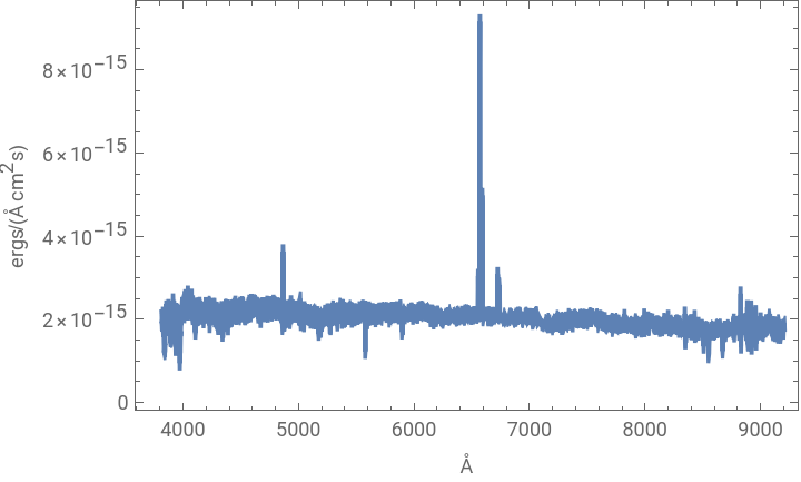
Plot the wavelengths versus the flux:
In[]:=
ListLinePlot[Transpose[{wavelengths,flux}],PlotRange->All,Frame->True,FrameLabel->{QuantityForm["Angstroms","Abbreviation"],QuantityForm["Ergs"/("Centimeters"^2"Seconds""Angstroms"),"Abbreviation"]}]
Out[]=
CITE THIS NOTEBOOK
CITE THIS NOTEBOOK
Plotting an Emission Line Spectrum from SDSS data
by Arnoud Buzing
Wolfram Community, STAFF PICKS, January 23, 2024
https://community.wolfram.com/groups/-/m/t/3107953
by Arnoud Buzing
Wolfram Community, STAFF PICKS, January 23, 2024
https://community.wolfram.com/groups/-/m/t/3107953