The study of phase transition is one of the most important aspects of condensed matter physics. It is concerned with classifying different phases of matter and the dynamics of a material/system to undergo phase transition from one phase to another. A famous result in this field is the Lee-Yang Theorem that indicates that and Ising-like system undergoes phase transition only in the absence of magnetic field (the theorem and the Ising models are discussed below). In this post, I will try to provide a computational approach to understanding/proving the Lee-Yang theorem.
Ising Model Phase Transition
Ising Model Phase Transition
The 2D Ising model is one of the most famous examples of ferromagnetism in physics. It consists of a collection of spins on lattice points, where the spin on site is labeled =±1. The nearest-neighbor spins interact with one another such that the magnetic energy of this bond is if they are aligned or if anti-aligned. In the presence of magnetic field , each spin contributes to the magnetic field. This means that the spins tend to align with the magnetic field to minimize the magnetic energy of the system. The magnetic energy of this system is thus given by ,where is the magnetization of the system. The ferromagnetic Ising model is known to undergo an order-disorder phase transition in the absence of a magnetic field. i.e. at high temperatures, the spins are almost randomly aligned resulting in zero magnetization (disordered phase). Upon lowering temperature, the interactions between spins start taking over and the system starts having finite magnetization (ordered phase). This is called a phase transition due to the discontinuous behavior of the magnetization as a function of temperature. This phase transition does not occur in the presence of magnetic field because the magnetization changes continuously. In literature, this discontinuous change appears as non-analyticity of the free energy of the system.
j
σ
j
-1
1
h
-
hσ
j
H=- -h
∑
〈ij〉
σ
i
σ
j
∑
j
σ
j
M=
∑
i
σ
i
Yang-Lee Theorem
Yang-Lee Theorem
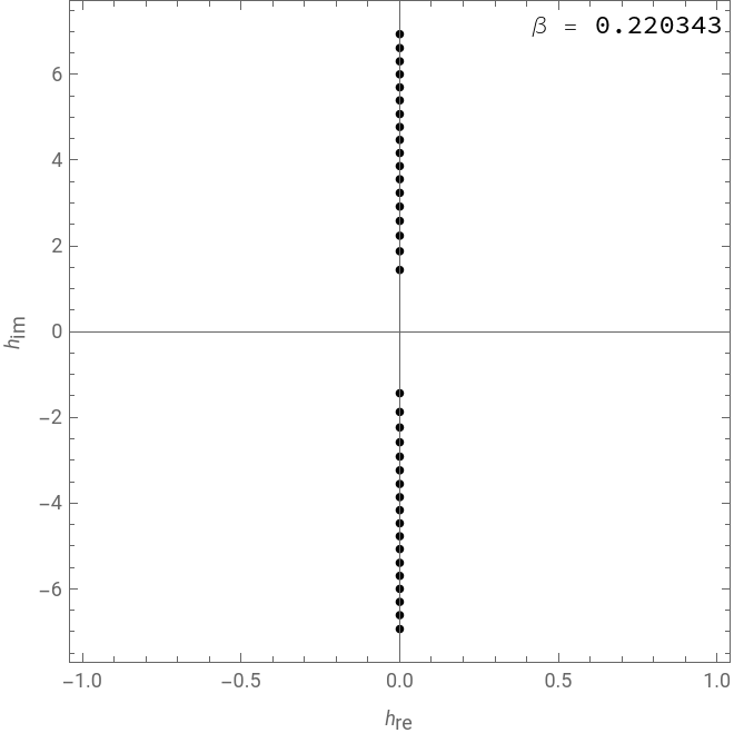
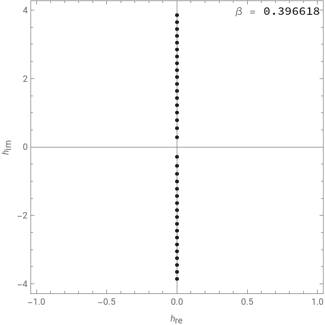
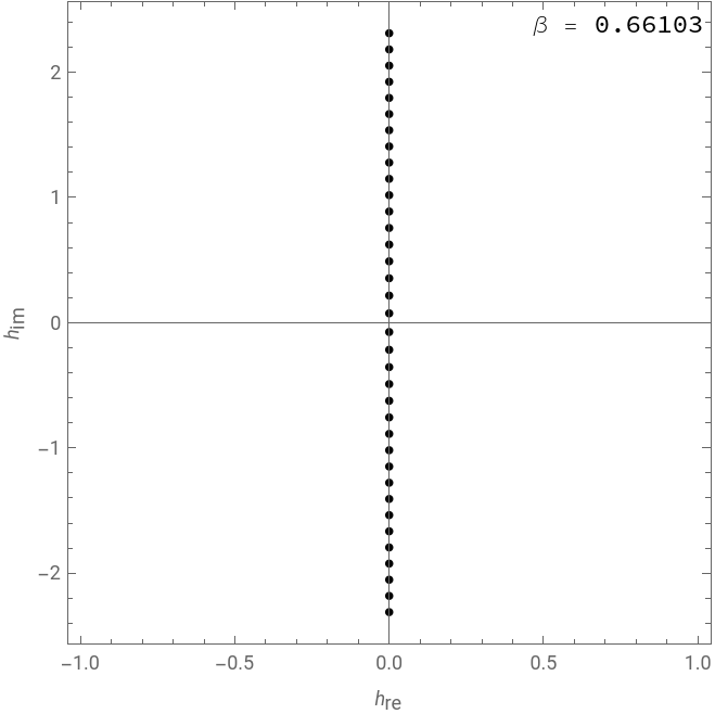
In 1952, Lee and Yang introduced a new way to study this phase transition through studying the zeros of the partition function because those zeros will correspond to non-analyticity of the free energy [1]. They proposed extending the magnetic field to take complex values such that where 1. The partition function is then given by ,where the sum is taken over all configurations and is the inverse temperature. They elegantly proved that, for ferromagnetic interaction, partition function vanishes only on the imaginary axis in the complex plane. i.e. the zeros of the partition function lie on the line 0This is infamous Lee-Yang Theorem. This theorem is valid for all dimensions, geometries, and long-range interaction. The only constraint is that the interactions have to be all ferromagnetic. The zeros of the partition functions are show in the pictures below. Disclaimer: The configurations were obtained from the exact diagonalization of the Ising model using Bhanot’s algorithm in an earlier project [2]. The powers of gives the magnetization, the power of gives the value of the interaction part of the energy, and the coefficients give the number of configurations with this magnetization and energy. The partition function was obtained for a shifted Hamiltonian; hence, the few products in front of the imported object.
Z
F∝-ln(Z)
h+i
h
re
h
im
2
i
Z(+i)
h
re
h
im
∑
{s}
-βH
e
∑
{s}
β+β
∑
〈ij〉
σ
i
σ
j
h
re
∑
j
σ
j
e
iβ
h
im
∑
j
σ
j
e
s
βT
1
k
B
(Z0)
h
h
re
Z(+i)0 ⟺ 0
h
re
h
im
h
re
z
u
In[]:=
Z=CloudGet[URLBuild[<|"Scheme""https","Domain""www.wolframcloud.com","Path"StringTemplate["obj/msedik7/Ising_PF_`l`x`l`_Open_BCs"][<|"l"->6|>]|>]];RowTableComplexListPlotLogz/.SolveNZ/.{u->},250==0,z,ImageSize->Medium,AspectRatio->1,Frame->True,FrameLabel->{"",""},PlotLegends->Placed[StringTemplate["β = `b`"][<|"b"->β//N|>],{Right,Top}],PlotStyle->Black,β,*Log[1+*Log[1+*Log[1+
1
2β
-2β
E
h
re
h
im
1
2
1
2
2
],9
10
1
2
2
],15
10
1
2
2
]Out[]=
Computational Approach
Computational Approach
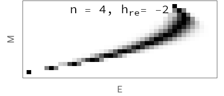
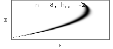
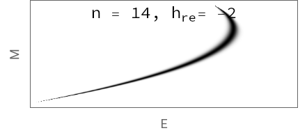
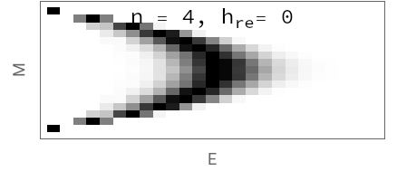
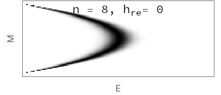
The goal of this note is to provide a computational view of the Lee-Yang theorem showing the reason why the partition function vanishes only on the imaginary axis 0 . We start by rewriting the partition function as , where the “energy” of a configuration is given by . The probability of having a magnetization is proportional to the sum over all configurations with this given . , and is the number of configurations with energy and magnetization . The partition function is then proportional to an expectation-value or (“thermal average”) of the phase factor of a random variable with some probability mass function (distribution) that depends on the temperature and the real part of the magnetic field. this averaging. Now we see that . Therefore, it suffices to show that one of the two “averages” is non-zero to make sure is not vanishing. We will focus on and provide a computational approach to show that it is unlikely to vanish when ≠0. We will consider a square array of spins. The pictures below are generated by considering all configurations with magnetization , then working out their distribution of energy , which is representative of the distribution of the magnetization.
Z
h
re
Z(+i)g(E,M)∝p(M)
h
re
h
im
∑
{s}
β+βM
∑
〈ij〉
σ
i
σ
j
h
re
e
iβM
h
im
e
∑
{s}
βE(s)
e
iβM
h
im
e
∑
E,M
iβM
h
im
e
βE
e
∑
M
iβM
h
im
e
s
E(s)--M
∑
〈ij〉
σ
i
σ
j
h
re
M
M
p(M)∝g(E,M)
∑
E
iβM
h
im
e
βE
e
g(E,M)
E
M
iβM
h
im
e
M
Z(+i)∝〈cos(βM)〉+i〈sin(βM)〉
h
re
h
im
iβM
h
im
e
h
im
h
im
whereindicates
〈...〉
Z0 ⟺ 〈cos(βM)〉0 and 〈sin(βM)〉0
h
im
h
im
Z
〈sin(βM)〉
h
im
h
re
nn
M
E
In[]:=
GridTableWitharray=CoefficientList2*(CloudGet[URLBuild[<|"Scheme""https","Domain""www.wolframcloud.com","Path"StringTemplate["obj/msedik7/Ising_PF_`l`x`l`_Open_BCs"][<|"l"->ntemp|>]|>]])/.{z->z},{z,u},With[{normArray=array/(Map[Max,array]/.{0->1})},ArrayPlot[normArray,FrameLabel->{"M","E"},ImageSize->Medium,PlotLegends->Placed[StringTemplate["n = `a`, = `b`"][<|"a"->ntemp,"b"->htemp|>],{Center,Top}],AspectRatio->1/2.5]],{htemp,{-2,0,2}},{ntemp,{4,8,14}}
ntemp(ntemp-1)/2+Abs[htemp]2
2
ntemp
u
2
ntemp
z
-ntemp(ntemp-1)/2
u
-2
2
ntemp
z
htemp
u
h
re
Out[]=
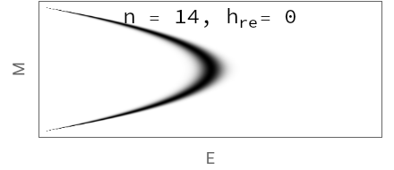
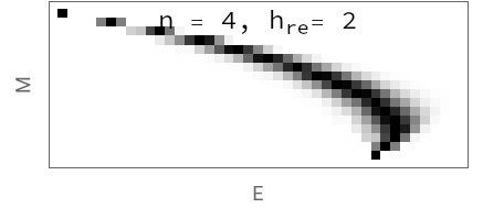
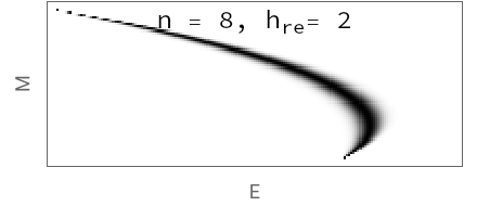
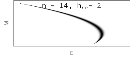
Numerical Experimentation
Numerical Experimentation
Conclusion
Conclusion
Future Direction
Future Direction
Acknowledgment
Acknowledgment
Credit is due to my advisor Professor Sriram Shastry for all the insightful discussion on the Lee-Yang zeros problem, and for the discussion on viewing the partition function as an ensemble average of the phase factor defined by imaginary part of the magnetic field. I also thank Professor Stephen Wolfram for suggesting studying the Lee-Yang theorem from a computational approach in this winter school.
References
References
[1] T.-D. Lee and C.-N. Yang, Statistical theory of equations of state and phase transitions. II. Lattice gas and Ising model, Phys. Rev. 87, 410 (1952).
[2] M. Sedik, J. M. Bhat, A. Dhar, and B. S. Shastry, “Yang-lee zeros of certain antiferromagnetic models,” Physical Review E, vol. 110, no. 1, p. 014117, 2024.
[2] M. Sedik, J. M. Bhat, A. Dhar, and B. S. Shastry, “Yang-lee zeros of certain antiferromagnetic models,” Physical Review E, vol. 110, no. 1, p. 014117, 2024.
CITE THIS NOTEBOOK
CITE THIS NOTEBOOK
Lee-Yang theorem and phase transitions - Computational approach
by Muhammad Sedik
Wolfram Community, STAFF PICKS, January 16, 2025
https://community.wolfram.com/groups/-/m/t/3358066
by Muhammad Sedik
Wolfram Community, STAFF PICKS, January 16, 2025
https://community.wolfram.com/groups/-/m/t/3358066