Problem definition (Choudhary et al. Commun Phys 5, 14 (2022))
Problem definition (Choudhary et al. Commun Phys 5, 14 (2022))
Microswimmers are micro-sized motile organisms (example: E. coli, Paramecium, Volvox, Chlamydomonas) that propel themselves via flagellar appendages or hair-like ciliary structure on their surface. The transport of these motile microorganisms is strongly influenced by fluid flows that are ubiquitous in biological environments. Here we demonstrate the impact of fluid inertia. We analyze the dynamics of a microswimmer in pressure-driven Poiseuille flow, where fluid inertia is small but non-negligible. Using perturbation theory and the reciprocal theorem, we show that in addition to the classical inertial lift of passive particles, the active nature generates a ‘swimming lift’, which we evaluate for neutral and pusher/puller-type swimmers. Accounting for fluid inertia engenders a rich spectrum of complex dynamics including bistable states, where tumbling coexists with stable centerline swimming or swinging. The dynamics is sensitive to the swimmer’s hydrodynamic signature and goes well beyond the findings at vanishing fluid inertia.The swimmer experiences (i.) self-propulsion velocity Vs (ii. ) background flow velocity (iii.) Far-field hydrodynamic and steric interactions with boundaries, (iv.) inertial lift (key aspect of the work). We assume that flow is 2D (Hele-Shaw geometry) and swimmer is not pointing out of the flow, and thus makes angle with the channel centerline. We also neglect thermal and athermal fluctuations.In this demonstration, we use neutral squirmer model which is applicable for swimmers like Paramecium and Volvox when made neutrally buoyant with surrounding fluid so that they swim force- and torque-free. Similar approach can be extended to Pusher/Puller type swimmers; refer the original article for further details on extension of this demo.
V
∞
θ
p
Inertial component via the Reciprocal theorem
Inertial component via the Reciprocal theorem
Here we are in the frame of reference of the swimmer. The notation here follows from the supplementary material of the cited article.
Essentially, we use the reciprocal theorem to find the correction to swimmer’s dynamics. Equation 3 suggests that it is a volume integral over the fluid domain in Stokesian limit.
Essentially, we use the reciprocal theorem to find the correction to swimmer’s dynamics. Equation 3 suggests that it is a volume integral over the fluid domain in Stokesian limit.
In[]:=
ClearAll["Global`*"]
(*Quit[]*)V∞={0,0,βX}-{VsSin[θp],0,VsCos[θp]}//Simplify;
Background velocity relative to swimmer' s self - propulsion at zeroth order . Eq . 16
Below are the coefficients of the disturbance velocity caused by the swimmer in Stokesian limit. These can be obtained from the literature or from well-known Lamb's general solution.
Below are the coefficients of the disturbance velocity caused by the swimmer in Stokesian limit. These can be obtained from the literature or from well-known Lamb's general solution.
B1z=;B1x=;
VsCos[θp]
2
VsSin[θp]
2
θp is the clockwise angle made in the first quadrant. To be consistent with the article, at the end of this section we will replace with π+ψ, where ψ is in the third quadrant.
θ
p
D1=β;EE1=β;Rvec={X,Y,Z};(*radiusvector*)eX={1,0,0};(*unitvector*)eZ={0,0,1};(*unitvector*)
-5
2
-1
2
Disturbance velocity
v01=(B1x)-++(B1z)-++D1+EE1ZeX+XeZ-/.{RSqrt[++]};
eX
3
R
3XRvec
5
R
eZ
3
R
3ZRvec
5
R
ZXRvec
5
R
5XZRvec
2
R
1
5
R
2
X
2
Y
2
Z
TestfieldEq.15:denotedasintext
t
u
u1=eX++eX-/.{RSqrt[++]};
3
4
XRvec
2
R
1
R
1
4
3XRvec
2
R
1
3
R
2
X
2
Y
2
Z
The integrand is divided in two parts: terms coming from the interaction of undisturbed and disturbed fields, and those purely from disturbed fields.
Integrand of Interaction
ITGDint=u1.(v01.Transpose[Grad[V∞,{X,Y,Z},"Cartesian"]]+V∞.Transpose[Grad[v01,{X,Y,Z},"Cartesian"]])//Simplify;
Integrand of pure disturbances
ITGDdist=u1.(v01.Transpose[Grad[v01,{X,Y,Z},"Cartesian"]])//Simplify;
Interaction term
Interaction term
In[]:=
sphINT=Simplify[(ITGDint)/.{XrSin[θ]Cos[ϕ],YrSin[θ]Sin[ϕ],ZrCos[θ]}];(*integrandinsphericalcoordinates*)INTpsi=(sphINT)Sin[θ]ϕ;INTtheta=INTpsiθ;INTrad=INTthetar;
2π
∫
0
2
r
π
∫
0
∞
∫
1
Disturbance term
Disturbance term
Integrand in spherical coordinates
sphDIST=Simplify[(ITGDdist)/.{XrSin[θ]Cos[ϕ],YrSin[θ]Sin[ϕ],ZrCos[θ]}];DISTpsi=(sphDIST)Sin[θ]ϕ;DISTtheta=DISTpsiθ;DISTrad=DISTthetar;
2π
∫
0
2
r
π
∫
0
∞
∫
1
Total
Total
Coefficient in front of integral. We obtain the inertial correction for the neutral swimmer; See methods section Eq. 17
-1
6π
Out[]=
7
24
Linear Stability Analysis
Linear Stability Analysis
Here we perform LSA by finding the eigenvalues of the system of two equations temporal differential equations: (i.) , (ii)
x
ψ
Stokes (Zottl and Stark 2012 Phys. Rev. Lett. 108, 218104)
Stokes (Zottl and Stark 2012 Phys. Rev. Lett. 108, 218104)
In[]:=
ClearAll["Global`*"]
In[]:=
jac={{D[vfx,ψ],D[vfx,x]},{D[-Sin[ψ],ψ],D[-Sin[ψ],x]}};jac//MatrixForm(*Jacobian*)λI=Eigenvalues[jac]/.{ψ0,x0}//SimplifyλII=Eigenvalues[jac]/.{ψ0,xπ}//Simplify
Out[]//MatrixForm=
0 | vf |
-Cos[ψ] | 0 |
Out[]=
-
vf
,vf
Out[]=
-
vf
,vf
Inertia
Inertia
In[]:=
jac={D[vfx,ψ],D[vfx,x]},D-Sin[ψ]+RePvfκx1--xCos[ψ],ψ,D-Sin[ψ]+RePvfκx1--xCos[ψ],x//Simplify;jac//MatrixForm(*Jacobian*)λI=Simplify[Eigenvalues[jac]/.{ψ0,x0},x0∈Reals&&x0>0];λII=Simplify[Eigenvalues[jac]/.{ψπ,x0},x0∈Reals&&x0>0];λI/.{ReP,vf}λII/.{ReP,vf}
2
x
2
x0
2
x
2
x0
Re
p
v
m
Re
p
v
m
Out[]//MatrixForm=
0 | vf |
-Cos[ψ]+RePxSin[ψ] | RePvf1- 3 2 x 2 x0 |
Out[]=
(-1+κ)-(-1+κ)+
1
2
Re
p
v
m
-4+
,v
m
2
Re
p
2
(-1+κ)
v
m
1
2
Re
p
v
m
-4+
v
m
2
Re
p
2
(-1+κ)
v
m
Out[]=
+κ-+κ+
1
2
Re
p
Re
p
v
m
4+
,v
m
2
(+κ)
Re
p
Re
p
v
m
1
2
Re
p
Re
p
v
m
4+
v
m
2
(+κ)
Re
p
Re
p
v
m
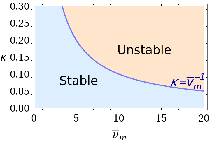
Downstream swimming corresponds to a saddle fixed point (λ2), while upstream swimming along the centerline (λ1) is stable for weak flows ) and unstable otherwise. The inertial lift profile plotted in Fig. 2 for a moderate flow strength and for different swimmer orientations ψ, shows the passive lift velocity at ψ = π/2 with an unstable position in the center and the two inertial focusing points at ±xeq. In the presence of the swimming lift, the centerline position is stabilized at ψ = 0. For strong flows(>) the centerline position becomes unstable. However, the swimmer cannot focus on a non-zero x position, because due to the non-zero vorticity of the Poiseuille flow, it continuously tumbles while drifting downstream.
(<
v
m
-1
κ
v
m
-1
κ
In[]:=
align[Center]={0,0};(*default*)align[Right]={-1,0};UText=Text[Style["Unstable",21,"Times New Roman"],{13,0.17},align[Center]];SText=Text[Style["Stable",21,"Times New Roman"],{3,0.08},align[Right]];EQText=Text[Style["κ=",21,"Times New Roman",Darker[Blue]],{16,0.078},align[Right]];txt=Graphics[{SText,UText,EQText}];Show[ContourPlot[Re[λI/.{ReP0.1}][[1]],{vf,0.1,20},{κ,0,0.3},ContourStyle{Blue},FrameTicksStyleDirective[Black,18],FrameLabel{Style["",20],Style["κ",20]},LabelStyle{FontSize18,FontFamily"Times New Roman",Black},ContourShading{LightBlue,LightOrange},Contours{0},RotateLabelFalse,ImageSizeMedium,AspectRatio0.6,BaseStyleThick],txt]
-1
v
m
v
m
Out[]=
Trajectories of neutral swimmer
Trajectories of neutral swimmer
Steric wall-repulsion
Integration module of eq .1
Coexisting states
Coexisting states