Goals of the Project: Torsion of a connection has been studied as the substrate for matter gauge field since the early days of Einstein-Cartan Theory. In this work we aim to study the minimal form of the ideas shared in such theory, on the setting of the graph rewrite system, where torsion is identified with topological defects. The analysis of different topological defects and their possible dynamics in a two dimensional flat background are aim to be described and hopefully find particle-like behaviour of defects and internal gauge degrees of freedom.
Main result: a plausible interaction between topological defects is defined in a centered hexagonal grid where these can be regarded as particles and an infinite range interaction field is analyzed. The computational tools for further study have been also created.
Future Work: now that the setup of the interaction is established and the computational tools are created, many interesting experiments can be done to analyze the behaviour of the defects and see 1) how the interaction works in different scenarios and 2) how well does this behaviour match with nature. Before jumping into 3D grids, there are many things left to analyze like many defect problems, rotation of defects, defects with different nature (possibly symmetric), etc.
Main result: a plausible interaction between
D
5
D
7
Future Work: now that the setup of the interaction is established and the computational tools are created, many interesting experiments can be done to analyze the behaviour of the defects and see 1) how the interaction works in different scenarios and 2) how well does this behaviour match with nature. Before jumping into 3D grids, there are many things left to analyze like many defect problems, rotation of defects, defects with different nature (possibly symmetric), etc.
Introduction
Introduction
In most modern theories of physics nature is described by spacetime, a four dimensional smooth manifold, where concepts from differential geometry like curvature and torsion play a key role describing interactions like gravity. Wolfram models, however, use discrete structures (hypergraphs) to describe nature and build physical laws on it, and hence, this differential geometry objects have to be translated to discrete metric spaces. By doing this in a proper way, hopefully, particle-like behaviour, interactions and gauge fields might come out in a natural way.
There are different ways of detecting curvature on a graph, but let me work on this first approach, which I find very natural. There are only three ways of tiling a two-dimensional flat space by regular polygons: four squares, three hexagons and six equilateral triangles in each vertex. Only the triangular grid (or centered hexagonal grid) has all the closest vertices at the same distance though, plus, it can be really easily constructed from the other two just by adding edges and vertices.
There are different ways of detecting curvature on a graph, but let me work on this first approach, which I find very natural. There are only three ways of tiling a two-dimensional flat space by regular polygons: four squares, three hexagons and six equilateral triangles in each vertex. Only the triangular grid (or centered hexagonal grid) has all the closest vertices at the same distance though, plus, it can be really easily constructed from the other two just by adding edges and vertices.
In[]:=
GraphicsGrid[{{GridGraph[{4,4}, ImageSizeSmall], ResourceFunction["HexagonalGridGraph"][ {3,3},ImageSize Small],ABCGraph[3]}}]
Out[]=
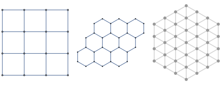
Pentagons, for example, do not tile the two-dimensional flat space, since the angle of each vertex is of 108º and can not sum 360º. However, if the grid is positively curved the angles of a pentagon get wider and can indeed appear in the grid. Having a centered hexagonal grid, the existence of a pentagon is an indication of positive curvature (similarly, an heptagon is a sign of negative curvature).
In[]:=
sph=DiscretizeGraphics[Graphics3D[Sphere[]]];DiscreteSphere=MeshConnectivityGraph[sph,VertexShapeFunction"Point",EdgeShapeFunction"Line"];HighlightGraph[DiscreteSphere,{NeighborhoodGraph[DiscreteSphere,{0,12},1],{Style[NeighborhoodGraph[DiscreteSphere,{0,133},1],Purple]}}]
Out[]=

D5 and its Dynamics
D
5
At first it might look easy to define an update rule to describe the motion of a in the hex-grid. However, it is pretty complicated actually. Let me make some definitions first:
D
5
NON-PROPAGATING DYNAMIC RULE: it is a rule that defines the motion of a defect such that it does not generate more defects and it can be written by a finite set of rules even if the graph is infinite.
It is quite obvious that a non-propagating dynamic rule has to be able to be executed within a closed subgraph, and hence the search of a non-propagating dynamic rule can be reduced to the search of a rearrangement of the interior of the subgraph that also generates a single defect (in a different position), without changing the nature of the boundary. By “without changing the nature of the boundary”, I mean that if a vertex belonging to the boundary has a certain amount of edges towards the interior of the subgraph, after the arrangement this amount of edges has to be the same. This must be obeyed, otherwise, that vertex would generate a defect after the rearrangement.
In[]:=
DD5=Graph[EdgeList[NeighborhoodGraph[DiscreteSphere,{0,12},6]],VertexLabelsAutomatic,ImageSizeLarge];li=VertexList[DD5][[All,2]];D5=VertexReplace[DD5,Table[{0,li[[i]]} i,{i,1,Length[li]}]];HighlightGraph[D5,{Style[{2527,2551, 5145, 4511,1144,4466,6615,1567,6760, 6039,3959,5956,5632,3230,3089,8927 },Blue],Style[{6,2,3,4,5,62,23,34,45,56},Red]}]
Out[]=
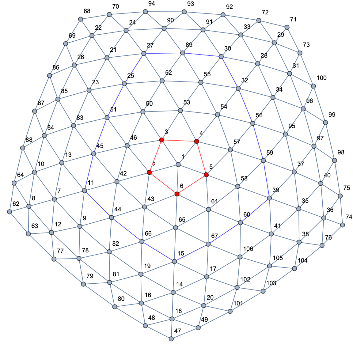
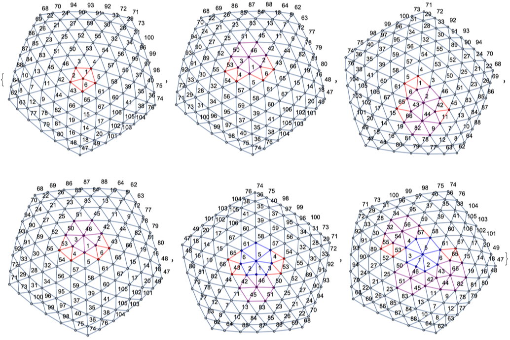
It is not difficult to see that due to the presence of the defect the nature of the boundary is not symmetric (in the direction of the defect), which makes a non-propagating dynamic rule very difficult to find (without loosing the nonplanarity). I think there might not even exist such a rule, no matter how big (non-infinity) the boundary is taken to be. Nevertheless, this suggests that there are non-propagating dynamics rules for pairs of defects (which of course can be drawn inside a symmetric boundary). All the dynamic rules I have attempt generate inevitably more defects. Here there is one example:
Coordinate system for centered hexagonal grids
Coordinate system for centered hexagonal grids
The coordinate system we are going to use in the centered hexagonal grid is the Cubic Coordinate system, which is obtained from a cubic grid by slicing out the diagonal plane x+y+z=0. This way there are three directions on the grid, and of course one of them is redundant. However, it is convenient to keep them all since we know that the sum of all three coordinates of any vertex in the hex-grid will sum zero. We have created some functions to play with this coordinate system, equipped with a very useful set of options. Here we have some examples of what we can do with them:
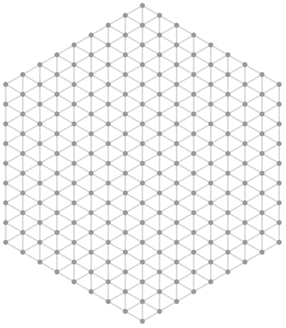
Create a hex-grid of desired radius with the Cubic Coordinate system ToolTip:
Create a hex-grid of desired radius with the Cubic Coordinate system ToolTip:
In[]:=
ABCGraph[8]
Out[]=
Use colors to indicate the values of the coordinates:
Use colors to indicate the values of the coordinates:
In[]:=
GraphicsGrid[{{ABCGraph[3,ColorFunctionExtract[1]],ABCGraph[3,ColorFunctionExtract[2]],ABCGraph[3,ColorFunctionExtract[3]]}}]
Out[]=
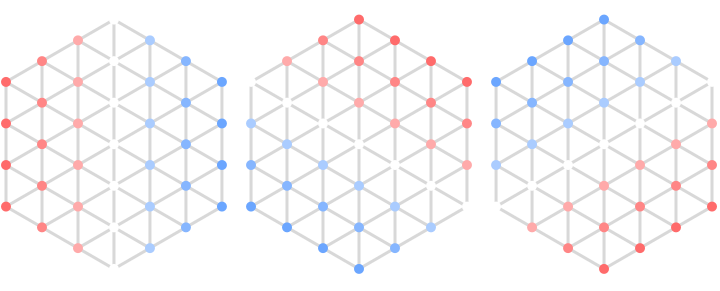
Label the coordinates directly:
Label the coordinates directly:
In[]:=
ABCGraph[2,LabelingFunctionFunction[#],ImageSizeMedium]
Highlight a specific vertex or list of them:
Highlight a specific vertex or list of them:
Zip dynamics?
Zip dynamics?
The process of stitching a rift is very similar to closing a zipper. The defect acts like the head of a zipper in the sense that when it moves in one direction it opens the jacket (in our case it generates a new rift) and when it moves in the opposite direction it closes it, bringing both edges of the rift together and closing it. It is literally like stitching.
In this illustrations the purple path indicates the chosen rift, the yellow point is the center of the pentagon, the green point is the center of the heptagon. Highlighted black pair of edges are the edges that have been stitched in the previous step and the shadowed parallelogram is the area is going to be stitched in the next step.
Strength of the interaction
Strength of the interaction
What can we say about this set up for interactions between topological defects?
What can we say about this set up for interactions between topological defects?
Well, this set up has many interesting properties one could analyze and compare with known physics in continuous spacetime, as well as some problems. Let me write down some of them.
There are many simulations and experiments to be done yet, and now that the complicated tool for that have been created, this ideas can be computed and analyzed much further.