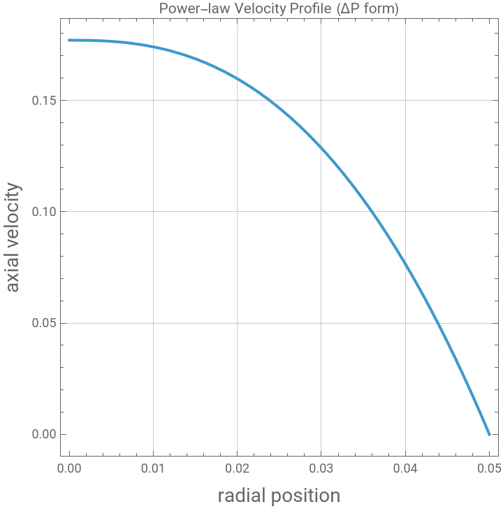
This notebook demonstrates an inverse problem in non-Newtonian fluid mechanics: recovering the rheological parameters of a power-law fluid — the consistency index K and flow behavior index n — from noisy experimental velocity measurements, using Particle Swarm Optimization as a curve-fitting method. The forward model describes the axial velocity profile v(r) for pressure-driven laminar flow of a power-law fluid through a pipe of radius R = 0.05 m under a pressure drop of 5000 Pa over a 50 m length, with the analytical velocity profile derived from the generalized Navier-Stokes equation for shear-thinning fluids (n = 0.65, K = 0.6).
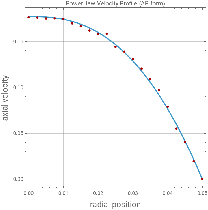
The notebook first generates a clean theoretical velocity profile, showing the characteristic blunted, plug-like shape typical of shear-thinning fluids — flatter near the pipe centerline and dropping off sharply near the wall compared to a parabolic Newtonian profile. Synthetic “experimental” data is then created by sampling this profile at 21 radial positions and adding small random noise (±0.005) using a seeded random generator for reproducibility, mimicking the kind of measurement scatter one would encounter in a real rheometry or flow visualization experiment.
With the true parameter values deliberately cleared from memory, the inverse problem is posed as a least-squares fitting task: find the K and n values whose predicted velocity profile best matches the noisy data points, using a fitness function that sums squared residuals between model and measurements across all 21 data points. This is treated as a 2D optimization problem over a search domain of {K,n} ∈ [0.01, 3.0]×[0.0, 2.5], a fairly wide search space given the risk of local minima and parameter correlation common in rheological curve-fitting problems.
PSO optimizer is used with 30 particles over 1000 iterations, tracking convergence every 20 iterations. The loss drops quickly within the first 100 iterations from around 0.000115 to 0.0001134, then plateaus almost perfectly for the remaining 900+ iterations — a strong signal that the swarm has converged to a well-defined minimum in parameter space, aided by the smoothness of the least-squares objective near the true solution.
The recovered parameters, K ≈ 0.638 and n ≈ 0.614, closely match the true underlying values (K = 0.6, n = 0.65) despite the fit being performed on noisy synthetic data, confirming that PSO can reliably back out physically meaningful rheological constants from experimental-style measurements.
Finally, the convergence plot, shown on a log scale, captures the characteristic rapid-then-flat PSO trajectory, while a direct check of the fitness function at the true parameter values (0.6, 0.65) yields a comparably small residual (≈0.000135), confirming the noise floor is consistent with the quality of the parameter recovery.
ClearAll["Global`*"]
Parameters
ΔP=5000;(*Pa*)L=50;(*m*)K=0.6;(*Pa.s^n*)n=0.65;R=0.05;(*m*)
Velocity profile
v[r_,K_,n_]:=(n/(n+1))*(ΔP/(2LK))^(1/n)*(R^((n+1)/n)-r^((n+1)/n));
Plot
p0=Plotv[r,K,n],{r,0,R},
Out[]=
In[]:=
SeedRandom[42];
In[]:=
data=Table[{r,Max[0,v[r,K,n]+RandomReal[{-0.005,0.005}]]},{r,0,R,R/20}]//Chop
Out[]=
{{0,0.176238},{0.0025,0.175801},{0.005,0.174937},{0.0075,0.175082},{0.01,0.174562},{0.0125,0.169627},{0.015,0.166618},{0.0175,0.161724},{0.02,0.157941},{0.0225,0.158398},{0.025,0.144104},{0.0275,0.138683},{0.03,0.13076},{0.0325,0.120228},{0.035,0.109016},{0.0375,0.0966837},{0.04,0.0789281},{0.0425,0.0552092},{0.045,0.0402936},{0.0475,0.0195685},{0.05,0.000281419}}
In[]:=
Show[p0,ListPlot[data,PlotStyle->Darker@Red]]
Out[]=
In[]:=
Clear[K,n]
PSO approach
In[]:=
Fitness[{K_,n_}]:=Sum[(v[data[[i]][[1]],K,n]-data[[i]][[2]])^2,{i,1,Length@data}];
2D problem
SwarmDim=2;
Upper and lower bounds for the search domain
FitnessLB={0.01,0.02};FitnessUB={3.0,2.5};
PSO parameters
c1=1.42;c2=1.42;w=0.72984;
Clip each column of a matrix against its own scalar bound
clipMatrix[mat_,lbv_,ubv_]:=Transpose[MapThread[Clip[#1,{#2,#3}]&,{Transpose[mat],lbv,ubv}]];clampMatrix[mat_,vmaxv_]:=Transpose[MapThread[Clip[#1,{-#2,#2}]&,{Transpose[mat],vmaxv}]];
PSO Optimizer
psoOptimize[lossFunc_,dim_,lb_,ub_,nParticles_:30,nIter_:100,wMax_:0.9,wMin_:0.4,c1_:1.42,c2_:1.42,vClampFrac_:0.2]:=Module[{particles,velocities,pbest,pbestScore,gbest,gbestScore,convergence={},r1,r2,scores,gbestIdx,vmax,wIter},vmax=vClampFrac*(ub-lb);particles=Transpose@Table[RandomReal[{lb[[i]],ub[[i]]},nParticles],{i,dim}];velocities=ConstantArray[0.,{nParticles,dim}];pbest=particles;pbestScore=lossFunc/@particles;gbestIdx=First@Ordering[pbestScore,1];gbestScore=pbestScore[[gbestIdx]];gbest=pbest[[gbestIdx]];Do[wIter=wMax-(wMax-wMin)*(j-1)/(nIter-1);r1=RandomReal[1,{nParticles,dim}];r2=RandomReal[1,{nParticles,dim}];velocities=wIter*velocities+c1*r1*(pbest-particles)+c2*r2*(ConstantArray[gbest,nParticles]-particles);velocities=clampMatrix[velocities,vmax];particles+=velocities;particles=clipMatrix[particles,lb,ub];scores=lossFunc/@particles;pbest=MapThread[If[#3<#2,#1,#4]&,{particles,pbestScore,scores,pbest}];pbestScore=MapThread[Min,{pbestScore,scores}];gbestIdx=First@Ordering[pbestScore,1];If[pbestScore[[gbestIdx]]<gbestScore,gbestScore=pbestScore[[gbestIdx]];gbest=pbest[[gbestIdx]];];AppendTo[convergence,gbestScore];If[Mod[j,20]==0,Print["PSO Iter ",j," Loss = ",gbestScore]];,{j,nIter}];{gbest,gbestScore,convergence}];
PSO run
result=psoOptimize[Fitness,SwarmDim,FitnessLB,FitnessUB,50,1000];{gbest,gbestScore,convergence}=result;
PSO Iter 20 Loss = 0.000114981
PSO Iter 40 Loss = 0.000114314
PSO Iter 60 Loss = 0.000114314
PSO Iter 80 Loss = 0.000113561
PSO Iter 100 Loss = 0.000113552
PSO Iter 120 Loss = 0.000113549
PSO Iter 140 Loss = 0.000113484
PSO Iter 160 Loss = 0.000113464
PSO Iter 180 Loss = 0.000113427
PSO Iter 200 Loss = 0.000113427
PSO Iter 220 Loss = 0.000113427
PSO Iter 240 Loss = 0.000113427
PSO Iter 260 Loss = 0.000113427
PSO Iter 280 Loss = 0.000113427
PSO Iter 300 Loss = 0.000113427
PSO Iter 320 Loss = 0.000113427
PSO Iter 340 Loss = 0.000113427
PSO Iter 360 Loss = 0.000113427
PSO Iter 380 Loss = 0.000113427
PSO Iter 400 Loss = 0.000113427
PSO Iter 420 Loss = 0.000113427
PSO Iter 440 Loss = 0.000113427
PSO Iter 460 Loss = 0.000113427
PSO Iter 480 Loss = 0.000113427
PSO Iter 500 Loss = 0.000113427
PSO Iter 520 Loss = 0.000113427
PSO Iter 540 Loss = 0.000113427
PSO Iter 560 Loss = 0.000113427
PSO Iter 580 Loss = 0.000113427
PSO Iter 600 Loss = 0.000113427
PSO Iter 620 Loss = 0.000113427
PSO Iter 640 Loss = 0.000113427
PSO Iter 660 Loss = 0.000113427
PSO Iter 680 Loss = 0.000113427
PSO result vs . NMinimize solution
PSO convergence plot
CITE THIS NOTEBOOK
CITE THIS NOTEBOOK
Recovering rheological properties from noisy velocity data using PSO
by Housam Binous
Wolfram Community, STAFF PICKS, July 26, 2026
https://community.wolfram.com/groups/-/m/t/3745032
by Housam Binous
Wolfram Community, STAFF PICKS, July 26, 2026
https://community.wolfram.com/groups/-/m/t/3745032