The Wolfram Emerging Leaders Program: High School (WELP:HS) is a remote, semester-long program designed for exceptional graduates from the Wolfram High School Summer Research Program to continue to develop their skills. Students work in a small group over the course of a semester to do either a research-based project or a product development–based project under the guidance of expert mentors. Projects are centered around a topic at the intersection of the group’s interests.
Our research focuses on computationally modeling residential heating systems to understand how physical parameters govern heat loss, indoor temperature stability, and geothermal performance. Using a system-level energy balance framework, we modeled the indoor air temperature as a dynamic variable influenced by conductive losses through the building envelope, convective losses due to fluid and air exchange, and heat supplied by a geothermal borefield. Rather than prescribing heating behavior, the model allows indoor temperature and energy demand to emerge naturally from the interaction of coupled physical processes. Through a series of parametric simulations, we systematically varied wall thermal conductance, volumetric water flow rate, and subsurface geothermal temperature gradient to isolate their individual effects on system behavior. The resulting simulations and plots reveal how insulation and convection dominate short-term thermal response, while geological conditions ultimately constrain long-term heating performance. This work demonstrates how computational modeling can be used not only to simulate residential heating systems, but to reason about their physical limits and inform design decisions relevant to real-world geothermal heating applications.
Introduction and Hypothesis
Introduction and Hypothesis
Residential heating systems sit at the intersection of physics, engineering, and environmental constraints. While it is easy to say that “better insulation reduces heat loss” or that “geothermal systems are more efficient,” these claims only become meaningful when quantified. Computational modeling allows us to move beyond intuition and instead simulate how physical laws play out over time, under controlled assumptions, and across a range of parameters that would be difficult or expensive to test experimentally.
This project investigates how a residential heating system behaves when coupled to a geothermal heat source, with particular emphasis on how physical parameters control heat loss, indoor temperature stability, and long-term heating performance. The central hypothesis is that thermal performance is governed by a small set of dominant parameters: wall thermal conductance determines conductive heat loss, air exchange governs convective loss, and the subsurface temperature gradient controls geothermal heat availability. By systematically varying these parameters in a computational model, we aim to identify which mechanisms most strongly influence system behavior and why.
Rather than treating the model as a black box, this essay explains the mathematical structure of the system, the parameters available for manipulation, and the physical meaning of each simulation result, using plots and parametric studies as evidence for or against the hypothesis. To test this hypothesis, we constructed a custom system-level model and performed controlled computational experiments in which one physical parameter was varied at a time while all others were held constant.
Fundamental Heat Transfer Framework
Fundamental Heat Transfer Framework
At the core of every model used in this project is an energy balance applied to the indoor air volume. Rather than prescribing the indoor temperature as a fixed value, the model treats it as a dynamic state variable that evolves over time in response to competing heat gains and losses. This approach reflects physical reality: the temperature inside a building changes continuously as heat enters and leaves the space through the envelope, ventilation, and active heating systems. The governing equation for this balance can be written as
(/dt) = ( – ) + ( – ) +
This equation forms the mathematical backbone of every simulation presented later in this essay, including the final geothermal–building system model created for this project. Here, represents the effective thermal capacitance of the indoor air, which determines how quickly the indoor temperature responds to changes in heat flow. A larger thermal capacitance results in slower temperature variations, introducing thermal inertia into the system. The left-hand side of the equation therefore captures the rate at which thermal energy is stored or released by the indoor air as its temperature changes over time.
The first term on the right-hand side models conductive heat transfer through the building envelope. The wall thermal conductance aggregates material properties, wall thickness, and surface area into a single parameter that controls how easily heat flows through the walls. When the outdoor temperature is lower than the indoor temperature , this term becomes negative, representing heat loss from the room. Because the term is proportional to the temperature difference, it increases in magnitude during cold weather and for poorly insulated buildings.
The second term represents convective heat transfer due to air exchange between indoors and outdoors. This contribution depends on the mass flow rate of and the specific heat capacity of . Unlike conduction, which depends on wall properties, convective losses are driven by ventilation, infiltration, or leakage. This term is particularly important for transient behavior, as sudden changes in airflow can rapidly alter indoor temperature even when wall insulation remains unchanged.
The final term,, represents heat supplied by the hydronic heating system, which is ultimately driven by the geothermal borefield in the full system model. This term is controlled indirectly through system dynamics and control logic rather than being imposed directly. Wolfram System Modeler (WSM) solves this coupled differential equation numerically by integrating it with time-dependent weather data, component-level physical models, and control strategies.
c
air
dT
in
k
wall
T
out
T
in
m
air
c
air
T
out
T
in
Q
heat
This equation forms the mathematical backbone of every simulation presented later in this essay, including the final geothermal–building system model created for this project. Here,
c
air
The first term on the right-hand side models conductive heat transfer through the building envelope. The wall thermal conductance
k
wall
T
out
T
in
The second term represents convective heat transfer due to air exchange between indoors and outdoors. This contribution depends on the mass flow rate of
m
air
c
air
The final term,
Q
heat
Store the full model path for the geothermal borefield example.This model represents the subsurface heat exchanger that supplies thermal energy to the building heating system.
mm="AixLib.Fluid.Geothermal.Borefields.Examples.Borefields";
Load the System Modeler representation of the geothermal borefield.This exposes all equations,parameters,and state variables associated with ground heat extraction.
SystemModel[mm]
Out[]=
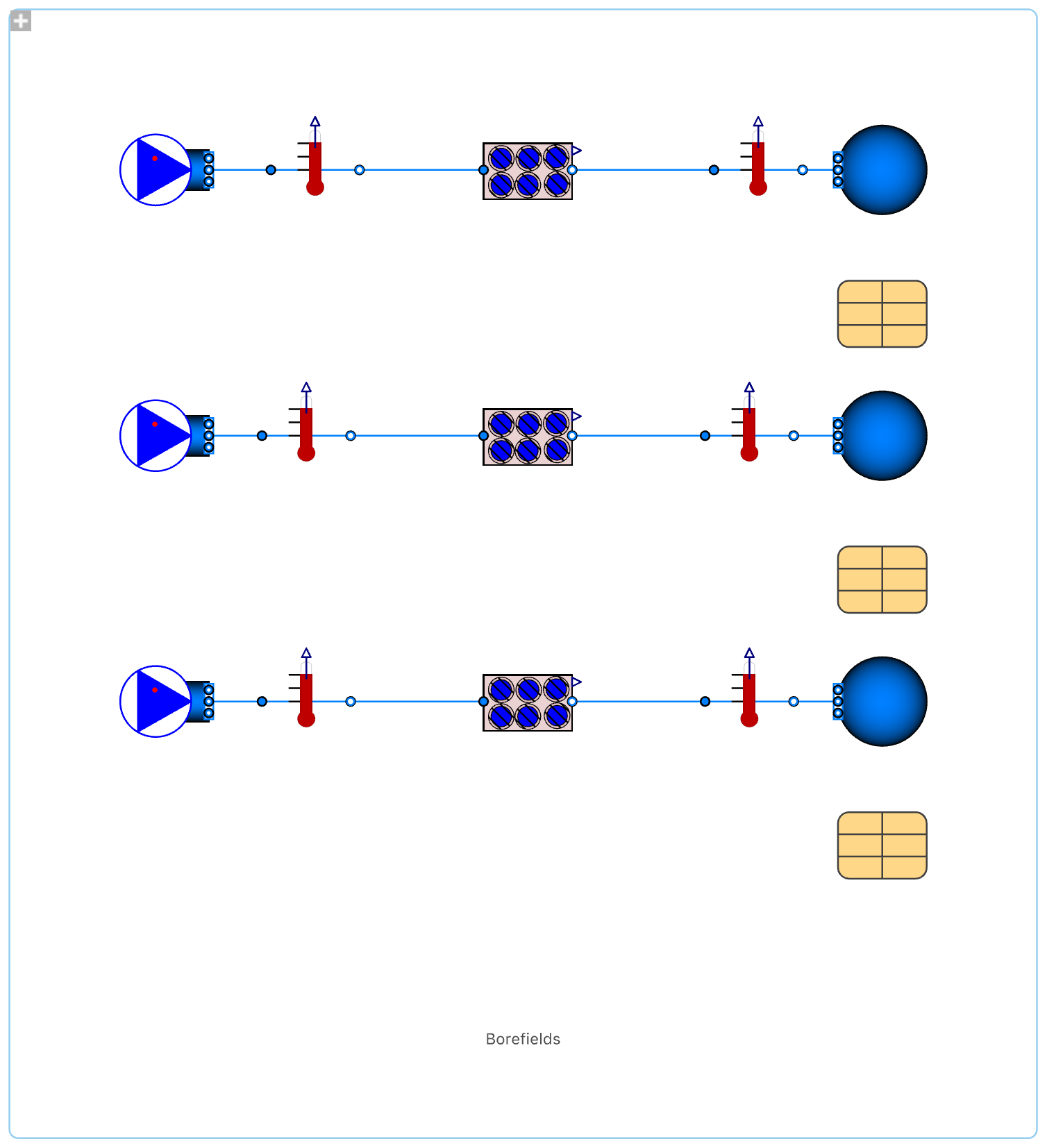
This command loads the geothermal borefield model that supplies heat to the building-side system analyzed throughout the remainder of the essay.
In[]:=
sim=SystemModelSimulate[mm];
Creating a simulation object exposes all model parameters and state variables for inspection and controlled modification.
As a result, the indoor temperature trajectory emerges naturally from the interaction of physical parameters rather than being enforced, making the model suitable for sensitivity analysis and parametric studies.
As a result, the indoor temperature trajectory emerges naturally from the interaction of physical parameters rather than being enforced, making the model suitable for sensitivity analysis and parametric studies.
Model Lineage: From Reference Examples to the Final Integrated System
Model Lineage: From Reference Examples to the Final Integrated System
The final model developed in this project did not emerge in isolation. Instead, it was informed by a sequence of progressively more complex reference models that clarified individual physical mechanisms before they were combined into a single system. Two existing models—SimpleHouse6 and HouseHeatingScenario—played a critical role in shaping the structure and parameterization of our final design, even though neither of them is the model ultimately analyzed.
SimpleHouse6 served as the foundational reference for understanding single-zone thermal dynamics.
In[]:=
SystemModel["AixLib.Examples.SimpleHouse"]
Out[]=
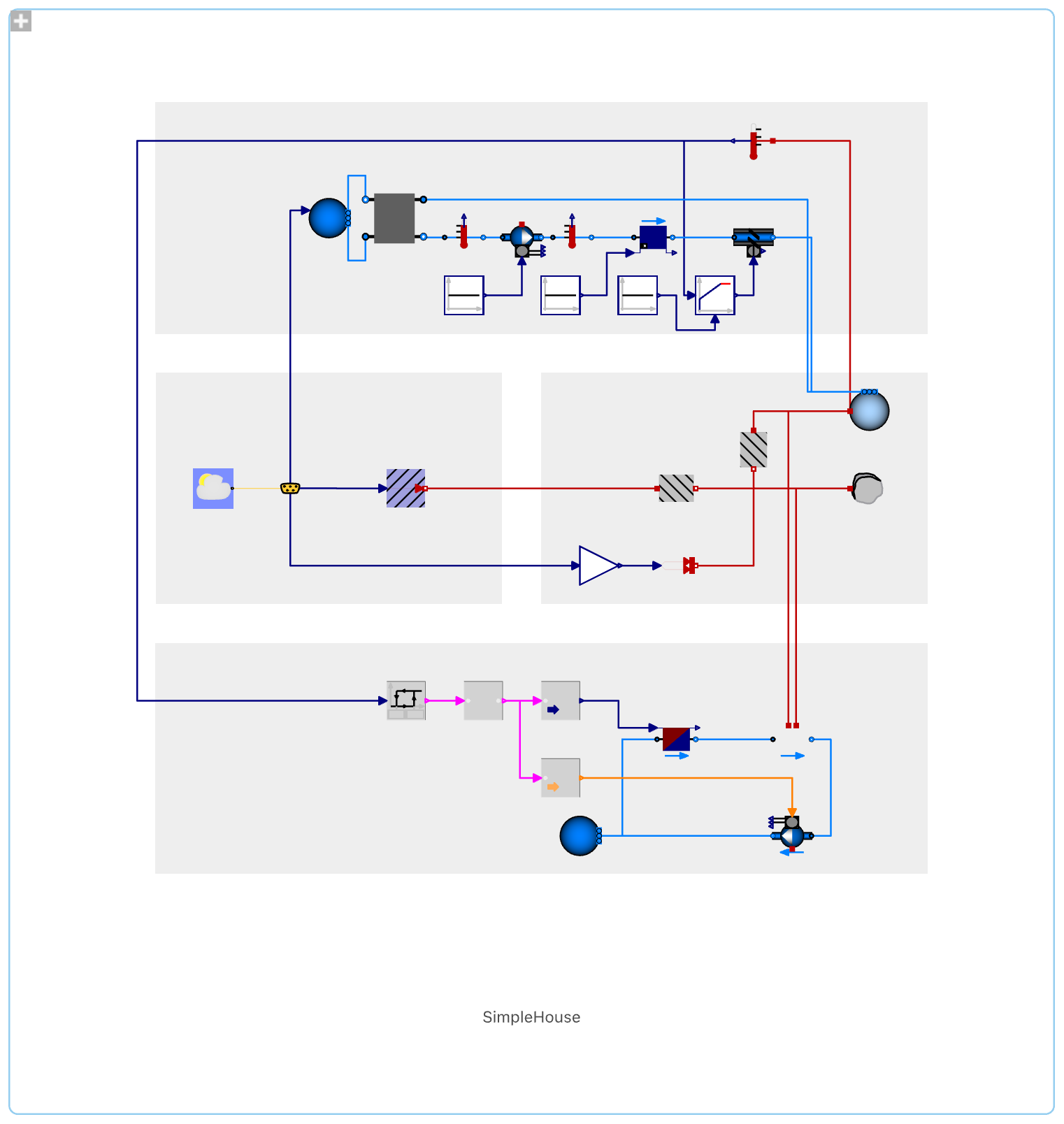
This model isolates the indoor air as a lumped thermal mass and explicitly represents heat loss through conduction and convection. From this model, we adopted the idea of representing the indoor space with a single energy balance equation, parameterized by wall conductance and air exchange rate. It also provided a clean framework for interpreting how insulation quality (via wall thermal conductance) and ventilation directly influence indoor temperature decay, which later guided our choice of parameters and test cases in the custom model.
The HouseHeatingScenario model extended these ideas by introducing control logic, weather forcing, and multi-component interaction.
The HouseHeatingScenario model extended these ideas by introducing control logic, weather forcing, and multi-component interaction.
In[]:=
SystemModel["IndustryExamples.Energy.HouseHeating.HouseHeatingScenario"]
Out[]=
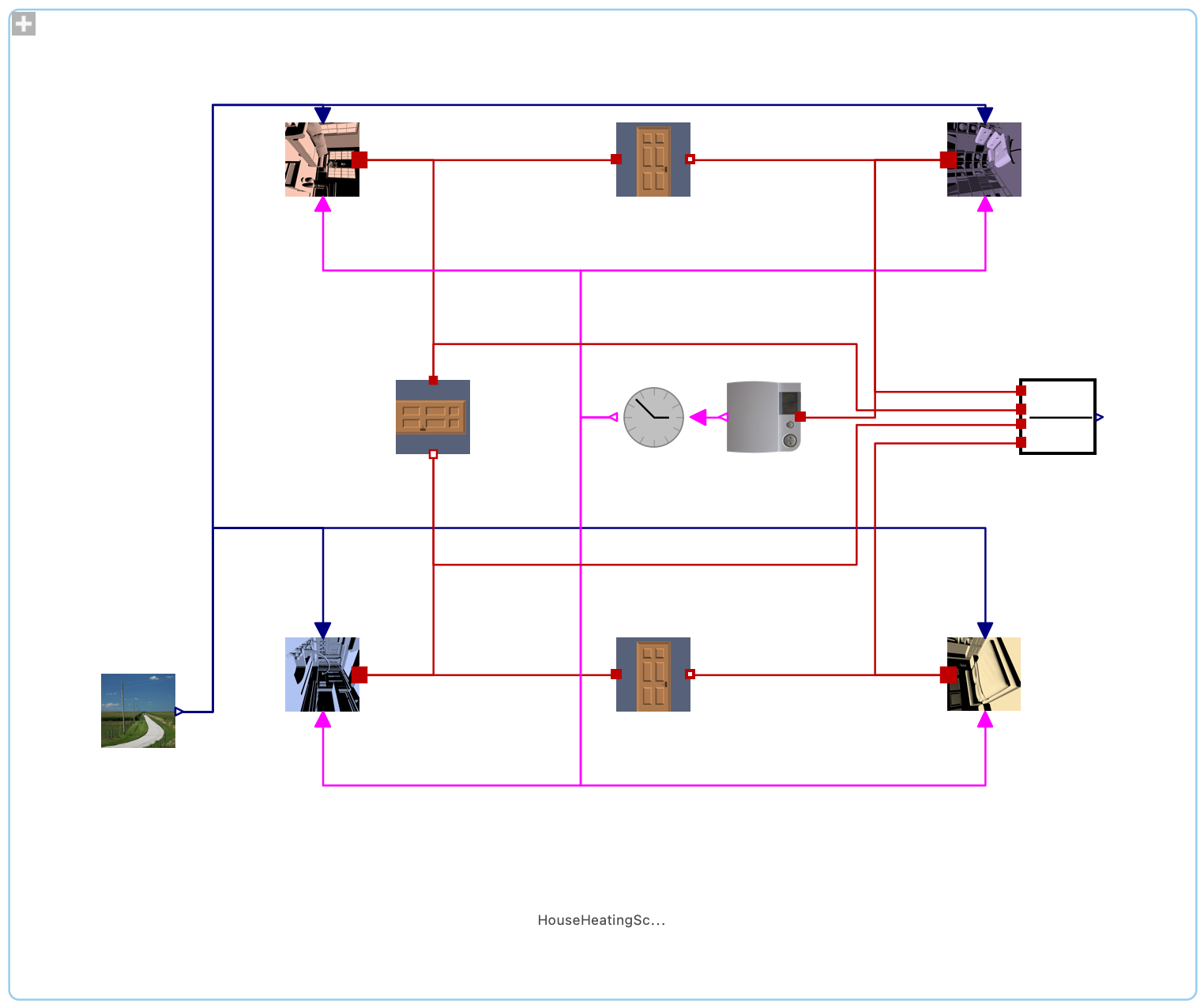
In this reference model, indoor temperature is no longer driven solely by passive losses, but also by an active heating system responding to thermostat logic and time schedules. This informed our decision to explicitly couple outdoor weather data, building thermal mass, and heating system dynamics in our own model, rather than prescribing indoor temperatures or heating power. The use of averaged indoor temperature for control, as well as the separation between physical heat transfer and control decisions, directly influenced how we structured the heating loop in our system.
Crucially, while these reference models guided our understanding of fundamental mechanisms, the final model shown in Figure X is a custom system built by us, integrating a geothermal borefield as the primary heat source. Neither SimpleHouse6 nor HouseHeatingScenario includes a geothermal subsystem; incorporating this component required new parameter choices, new couplings, and new analysis. The reference models provided physical intuition and validation checkpoints, but the final model represents a synthesis in which geothermal energy, building physics, and environmental forcing interact within a single framework.
All quantitative results and parametric studies presented in the remainder of this essay are generated exclusively from the final integrated model we developed, not from the reference example models.
Model Structure and Component Interactions
Model Structure and Component Interactions
The final system model brings together weather forcing, building thermal dynamics, a hydronic heating loop, and a geothermal heat source into a single coupled dynamical system.
simplecooling2 running on SystemModeler
Rather than modeling these elements in isolation, the model treats them as interacting subsystems whose behavior emerges from their physical connections.
Retrieve the names of all exposed physical parameters in the model. These include material properties, flow rates, thermal conductances, and geothermal soil characteristics.
The model exposes hundreds of tunable physical parameters, allowing precise control over building, fluid, and geothermal behavior. Outdoor temperature data provides time-varying boundary conditions, while the indoor thermal zone acts as an energy storage element whose temperature evolves according to conduction, convection, and active heating. This structure allows the model to respond realistically to changing environmental and operating conditions.
Retrieve the names of all state variables evolving over time. These include temperatures, pressures, mass flow rates, and heat transfer quantities throughout the system.
Display representative state variables that evolve dynamically
State variables include temperatures, pressures, mass flow rates, and heat transfer quantities evolving dynamically over time.
At the building level, the indoor zone is represented as a lumped thermal mass with finite heat capacity. Heat is exchanged with the environment through multiple parallel pathways. Conduction through walls and windows is driven by temperature differences between indoor and outdoor air, with wall and window conductances determining the magnitude of the heat flux. Ventilation and infiltration introduce convective heat transfer through mass flow of air, directly coupling outdoor conditions to the indoor energy balance. Together, these processes determine the baseline heating demand required to maintain thermal comfort.
The heating loop is modeled as a circulating fluid system that transfers energy from the geothermal source to the indoor space. A pump imposes mass flow through the loop, while pipes and a heat exchanger (or radiator) govern how thermal energy is delivered to the indoor air. The heat transfer rate depends on both the supply fluid temperature and the indoor air temperature, creating a feedback loop: as the room warms, the temperature difference across the heat exchanger decreases, reducing heat transfer. This feedback is essential for capturing realistic system behavior and transient responses.
The geothermal subsystem provides the upstream thermal input to the hydronic loop in the form of a time-dependent supply temperature.
Filter the list of state variables to identify quantities associated with the geothermal borefield outlet. Only string-valued variable names are considered to avoid symbolic evaluation errors.
These variables correspond to temperatures, pressures, and mass flows at the geothermal borefield outlet. This temperature depends on subsurface conditions, borefield depth, and soil thermal properties. Because the geothermal outlet temperature feeds directly into the heating loop, any variation in ground conditions propagates forward through the fluid circuit and ultimately affects indoor temperature. As a result, changes to geothermal parameters influence not just the heat source itself, but the entire building energy balance. Because each component exchanges temperature, heat flux, or mass flow data with its neighbors, no parameter change remains local; every modification propagates through the coupled system.
Conductive Heat Loss: Wall Parameter Sensitivity
Conductive Heat Loss: Wall Parameter Sensitivity
Convective Heat Exchange and Volumetric Water Flow Rate
Convective Heat Exchange and Volumetric Water Flow Rate
This outcome highlights the regulatory role of the hydronic loop: it does not simply deliver energy, but continuously redistributes it based on instantaneous temperature differences. Higher flow rates increase the system’s ability to regulate temperature by tightening the coupling between the indoor zone and the geothermal source. When the ground temperature is lower than the indoor air temperature, this coupling produces a mild cooling effect; when the ground is warmer, the same mechanism would provide heating. The direction and magnitude of heat transfer are therefore controlled jointly by geothermal conditions, fluid flow rate, and indoor thermal state.
Taken together, these results emphasize that effective temperature regulation in geothermal and hydronic systems depends on coordinated tuning of envelope properties, flow control, and subsurface conditions. The geothermal loop serves as a dynamic thermal regulator rather than a fixed heat source, and its interaction with indoor temperature can shift between heating and cooling regimes depending on operating conditions. Proper selection and tuning of flow rates is therefore essential for balancing responsiveness and energy efficiency in hydronic and geothermal heating systems.
Taken together, these results emphasize that effective temperature regulation in geothermal and hydronic systems depends on coordinated tuning of envelope properties, flow control, and subsurface conditions. The geothermal loop serves as a dynamic thermal regulator rather than a fixed heat source, and its interaction with indoor temperature can shift between heating and cooling regimes depending on operating conditions. Proper selection and tuning of flow rates is therefore essential for balancing responsiveness and energy efficiency in hydronic and geothermal heating systems.
Geothermal Heat Supply and Parametric Analysis
Geothermal Heat Supply and Parametric Analysis
The geothermal subsystem introduces an additional layer of physics by modeling heat extraction from the ground rather than heat exchange with the ambient air. Unlike conduction and convection losses, which depend on building parameters and weather conditions, geothermal performance is governed by subsurface thermal properties. In this model, the ground temperature profile is approximated using a vertical temperature gradient, dT/dz, which represents how temperature increases with depth below the surface.
Filter parameters to locate the vertical geothermal temperature gradient (dT/dz). This parameter controls how ground temperature increases with depth and limits available geothermal heat.
Create a parametric simulation with respect to the geothermal temperature gradient dT_dz. The parameter is treated symbolically and evaluated only at physically viable values.
This produces a parametric function mapping geothermal gradient values to time-dependent outlet temperatures.
Evaluate the parametric solution across a range of geothermal gradients to compare subsurface conditions. Each function represents a different soil temperature profile.
This allowed us to isolate the impact of subsurface temperature structure on the geothermal supply temperature without confounding effects from building parameters.
Plot all geothermal outlet temperature trajectories together.This visualization shows how higher temperature gradients lead to higher and more stable heat supply over time.
The resulting plot shows that higher geothermal gradients produce consistently higher and more stable outlet temperatures over the simulation period. In contrast, lower gradients lead to a more rapid decline in outlet temperature, indicating thermal depletion of the surrounding ground. This behavior reflects a reduced capacity of the soil to conduct heat toward the borehole at shallow gradients. These results demonstrate that geothermal system performance is fundamentally constrained by geological conditions, independent of insulation quality or ventilation strategy. As a result, even a well-designed building envelope cannot compensate for unfavorable subsurface thermal properties, reinforcing the importance of site-specific analysis in geothermal system design.
Linking Ground Behavior to Indoor Performance
Linking Ground Behavior to Indoor Performance
Conclusion
Conclusion
The results of these computational experiments provide direct evidence in support of the initial hypothesis regarding the dominant roles of envelope conduction, water exchange, and geothermal temperature gradient. This computational essay demonstrates that residential heating behavior emerges from tightly coupled physical processes rather than from any single component acting in isolation. By explicitly defining model parameters, identifying which quantities could be changed, and varying them systematically across simulations, the analysis revealed how energy flows propagate through the entire system. Wall thermal conductance governs steady conductive losses, air exchange rate controls transient sensitivity to outdoor conditions, and the soil temperature gradient constrains the maximum heating power available from the geothermal source.
The resulting plots—indoor temperature trajectories, parametric borefield outlet temperatures, and comparative time-series responses—provide direct evidence for the initial hypothesis: overall system performance is dominated by envelope losses and ventilation on short timescales, while long-term comfort and energy use are limited by subsurface thermal conditions. Rather than serving as isolated visual outputs, these graphs encode the physical consequences of each parameter choice and make trade-offs between insulation, ventilation, and geothermal capacity explicit.
Taken together, the results show how computational modeling enables not only simulation but physical reasoning. By coupling differential equations, empirical weather data, and component-level heat transfer models, the system reveals where design effort yields the greatest returns and where fundamental physical limits apply. This approach transforms the model from a descriptive tool into a predictive framework for evaluating residential heating strategies under realistic constraints.
Future Work
Future Work
1
.Include installation and operating cost estimates
2
.Expand geothermal ground modeling
3
.Add building geometry and zoning effects
4
.User-controlled insulation and ventilation inputs
5
.Compare geothermal to alternative heating systems
6
.Longer simulation time horizons
7
.Simplified performance metrics for users
8
.Geographic and climate sensitivity studies
9
.Sizing and design guidance
10
.More accessible visualization tools
Acknowledgments
Acknowledgments
Contributions from River Yu and Neil Ramarapu.
A huge thank you to our mentor, Shenghui Yang, for guiding us through this project and teaching us how to use SystemModeler. Also, thanks to Rory Foulger and the staff for hosting a great program this year!
A huge thank you to our mentor, Shenghui Yang, for guiding us through this project and teaching us how to use SystemModeler. Also, thanks to Rory Foulger and the staff for hosting a great program this year!
Bibliography
Bibliography
1
.Maier, Laura, David Jansen, Fabian Wüllhorst, Martin Kremer, Alexander Kümpel, and Tobias Blacha. “AixLib: an open-source Modelica library for compound building energy systems from component to district level with automated quality management.” Github. Last modified 2023. https://doi.org/10.1080/19401493.2023.2250521.
2
.“Modelica Fluid Examples.” Modelica. https://doc.modelica.org/Modelica%204.0.0/Resources/helpDymola/Modelica_Fluid_Examples_HeatExchanger_BaseClasses.html.
3
.O’Neill, Zheng. “Modelica-Based Dynamic Modeling of a SolarPowered Ground Source Heat Pump System: A Preliminary Case Study.” LiU Electronic Press. PDF.
4
.Wikipedia contributors. “First law of thermodynamics.” Wikipedia, The Free Encyclopedia. Last modified November 9, 2025. https://en.wikipedia.org/w/index.php?title=First_law_of_thermodynamics&oldid=1321327044.
5
.Wikipedia contributors. “Lumped-element model.” Wikipedia, The Free Encyclopedia. Last modified July 4, 2025. https://en.wikipedia.org/wiki/Lumped-element_model.
CITE THIS NOTEBOOK
CITE THIS NOTEBOOK
Analysis of heat loss in buildings and thermal performance of geothermal borefields
by Zamir Ashraf, and Alex Ning
Wolfram Community, STAFF PICKS, February 11, 2026
https://community.wolfram.com/groups/-/m/t/3638653
by Zamir Ashraf, and Alex Ning
Wolfram Community, STAFF PICKS, February 11, 2026
https://community.wolfram.com/groups/-/m/t/3638653