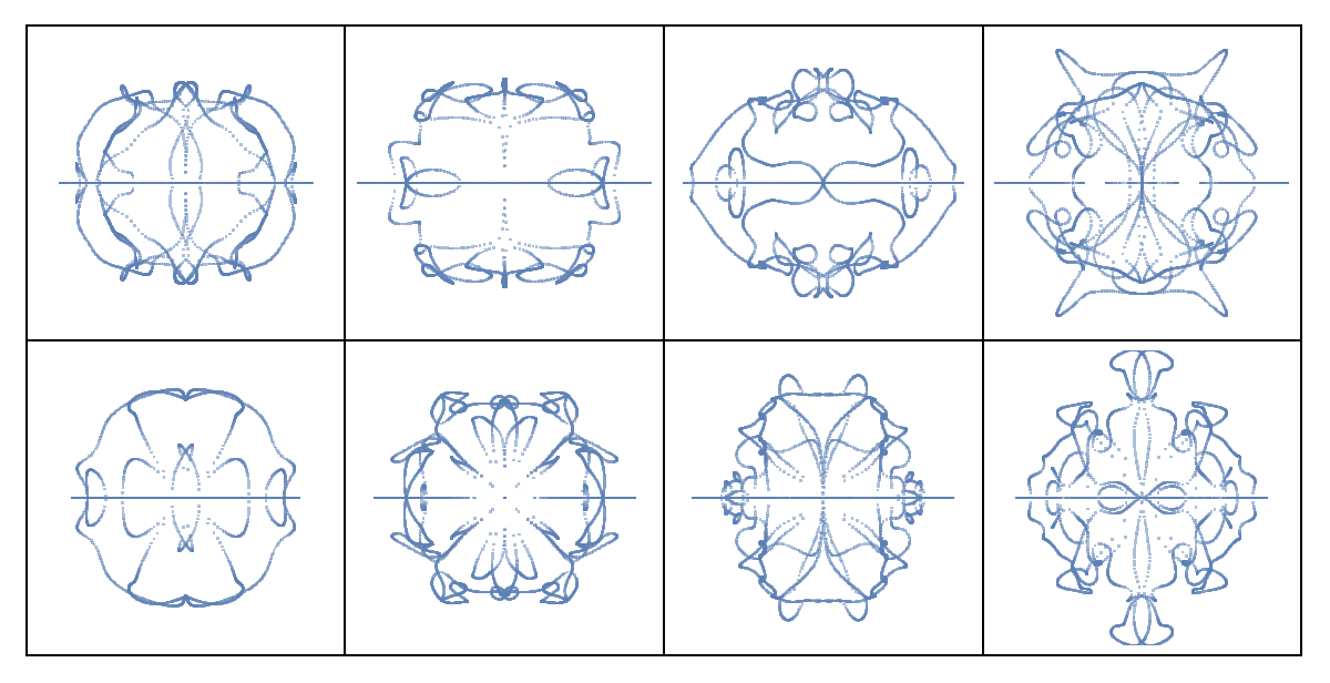
We can get an extra dimension to visualizing spectrum of the graph by visualizing the trajectory traced by its eigenvalues when we combine graphs adjacency matrix with an isoclinic rotation. Symmetry is provided by the fact that eigenvalues come in conjugate pairs, and an additional symmetry from the isolinic rotation.
In[]:=
Sat 11 Jan 2025 09:00:23
Uploading to newton/community-eigenvalue-graphs-trajectories.nb
ClearAll["Global`*"];SeedRandom[2];
Retrieve the Pappus Graph from GraphData
graph=GraphData["PappusGraph","Graph"];
Get the number of vertices in the graph
d=Length@VertexList@graph;
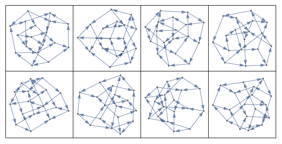
Define a function to create a grid of plots with a title
grid4[plots_,name_String]:=Column[{Style[Text[name],FontSize->Large,Bold],(*Titleabovethegrid*)With[{k=4}(*Numberofcolumnsinthegrid*),paddedPlots=PadRight[plots,Ceiling[Length[plots]/k]*k,Graphics[]];(*Padthelistofplotswithemptygraphicsifnecessary*)GraphicsGrid[Partition[paddedPlots,k],Frame->All](*Createagridofgraphics*)]},Alignment->Center]
Define a function to randomly assign direction to edges
randomDirection[a_b_]:=If[RandomReal[]<.5,ba,ab];
Generate 50 directed graphs with random edge directions
directedGraphs=Table[Graph[randomDirection/@EdgeList@graph],{50}];
Function to filter graphs with distinct spectra
GraphsWithDistinctSpectra[graphs_List]:=Module[{spectra},spectra=Sort/@(Eigenvalues[AdjacencyMatrix[#]]&/@graphs);Pick[graphs,Map[Count[spectra,#]==1&,spectra]]];
Filter the directed graphs to retain only those with distinct spectra
directedGraphs=GraphsWithDistinctSpectra[directedGraphs];
Display the directed graphs in a grid
grid4[directedGraphs,"Graphs"]
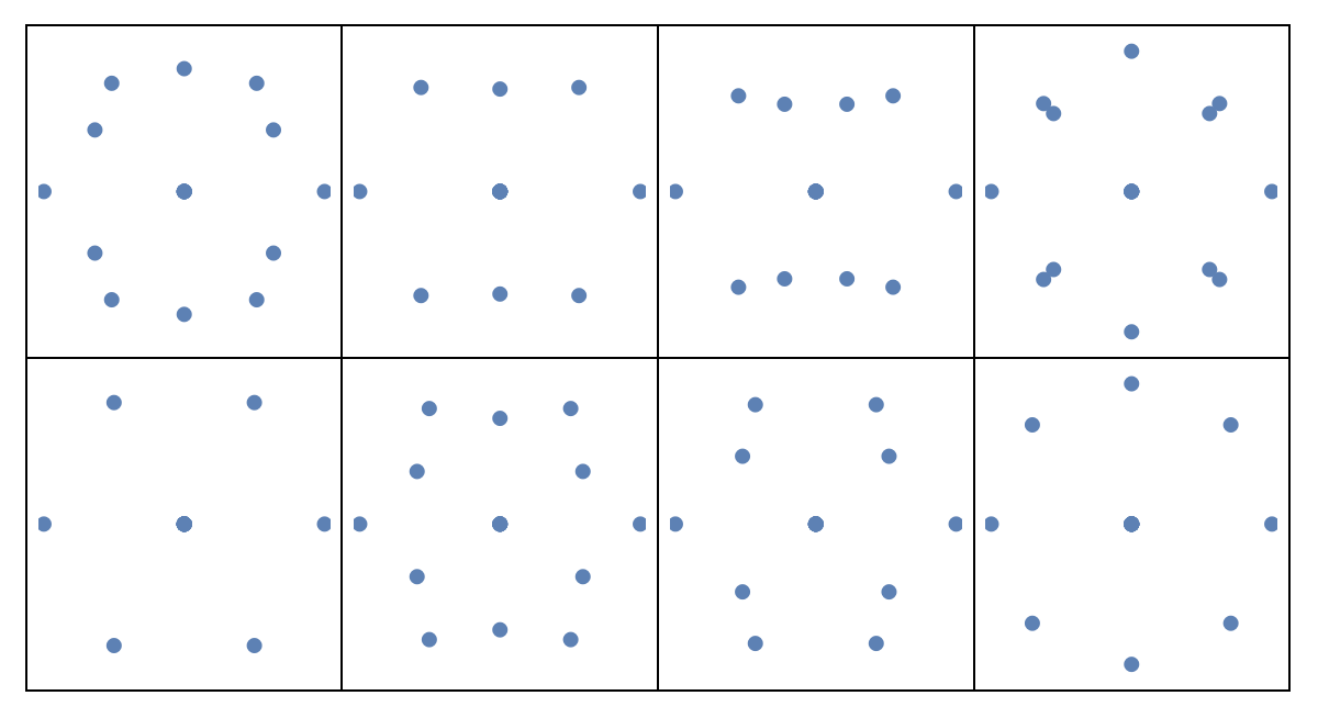
Compute eigenvalues for each directed graph
eigs=Table[Eigenvalues@AdjacencyMatrix@g,{g,directedGraphs}];
Plot the eigenvalues in the complex plane
plots=ComplexListPlot[#,PlotStyle->PointSize[Large],Axes->None]&/@eigs;
Display the eigenvalue plots in a grid
grid4[plots,"Eigenvalues"]
Define an isoclinic rotation function
isoclinic[theta_,P_]:=Module[{blocks,realJordanform,p,R,n},n=Length@P;blocks=Table[R[i]->RotationMatrix[theta],{i,n/2}];realJordanform=ArrayFlatten@(DiagonalMatrix[Array[R,n/2]]/.blocks);P.realJordanform.P(*Returntherotatedmatrix*)];
Function to generate and plot trajectories of eigenvalues under isoclinic rotation
genTraj[mat_,P_]:=With[{},evals=Table[Eigenvalues[isoclinic[theta,P].mat],{theta,0,2Pi,.02}];ListPlot[ReIm@Flatten@evals,PlotStyle->Directive[PointSize[.01],Opacity[.5]],PlotRange->{{-1.5,1.5},{-1.5,1.5}},AspectRatio->1,Axes->None]];
Generate and display trajectories for the directed graphs
plots=genTraj[Normal@AdjacencyMatrix@#,IdentityMatrix[d]]&/@directedGraphs;grid4[plots,"Trajectories"]
Out[]=
Graphs |
Out[]=
Eigenvalues |
Out[]=
Trajectories |
CITE THIS NOTEBOOK
CITE THIS NOTEBOOK
Trajectories of graph eigenvalues
by Yaroslav Bulatov
Wolfram Community, STAFF PICKS, January 11, 2025
https://community.wolfram.com/groups/-/m/t/3355240
by Yaroslav Bulatov
Wolfram Community, STAFF PICKS, January 11, 2025
https://community.wolfram.com/groups/-/m/t/3355240