ORIGINAL ARTICLE: Adam Cieślik, Eva Hackmann, and Patryk Mach: Kerr geodesics in terms of Weierstrass elliptic functions, Phys. Rev. D 108, 024056 (2023), DOI: https://doi.org/10.1103/PhysRevD.108.024056
Article Abstract: We derive novel analytical solutions describing timelike and null geodesics in the Kerr spacetime. The solutions are parametrized explicitly by constants of motion—the energy, the angular momentum, and the Carter constant—and initial coordinates. A single set of formulas is valid for all null and timelike geodesics, irrespectively of their radial and polar type. This uniformity has been achieved by applying a little-known result due to Biermann and Weierstrass, regarding solutions of a certain class of ordinary differential equations. Different from other expressions in terms of Weierstrass functions, our solution is explicitly real for all types of geodesics. In particular, for the first time the so-called transit orbits are now expressed by explicitly real Weierstrass functions.
Introduction
Introduction
Our paper introduces new general solutions to the Kerr geodesic equations in Boyer-Lindquist coordinates. These solutions are analytic and describe timelike and null geodesics in the Kerr spacetime. The solutions are explicitly parametrized by constants of motion, such as energy, angular momentum, and the Carter constant, along with initial coordinates. To simplify the usage of all the functions described in the paper, we have developed the KerrEqOfMotGeneral.wl package. In this notebook, I will demonstrate how to use it.
Install package
Install package
To use the KerrEqOfMotGeneral.wl package file in Mathematica, simply place it in the same directory as your notebook. Then, load the package using the below functions.
In[]:=
SetDirectory[NotebookDirectory[]];
In[]:=
<<"KerrEqOfMotGeneral.wl"
About functions in package
About functions in package
ThispackageprovidesgeneralsolutionsoftheKerrgeodesicequationsinBoyer-Lindquistcoordinates.Theyaregivenbythefollowingfunctions -ξ[s,{,,ε,κ,,α,δ}]-radialdistance; -θ[s,{,,ε,κ,,α,δ}]-polarcoordinate; -φ[s,{,,,,,ε,κ,,α,δ}]-azimuthalcoordinate; -Τ[s,{,,,,,ε,κ,,α,δ}]-timecoordinate;
ϵ
r
ξ
0
λ
z
ϵ
θ
θ
0
λ
z
φ
0
ϵ
r
ξ
0
ϵ
θ
θ
0
λ
z
Τ
0
ϵ
r
ξ
0
ϵ
θ
θ
0
λ
z
In order to obtain a complete description of a particular function, write:
?ξ
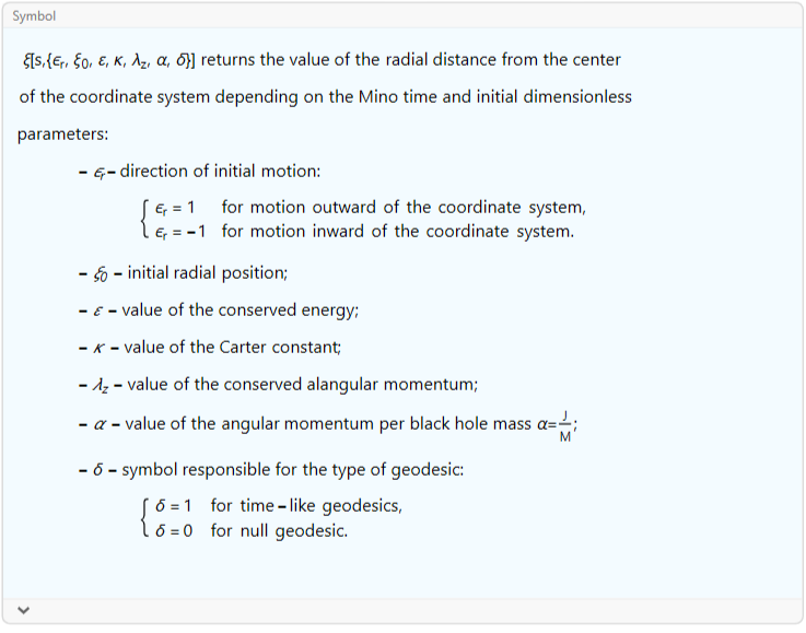
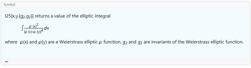
In addition to solutions to the equations of motion, the package also contains all integrals appearing in the work encoded, for example
?I1
?I25
?K3
?L3
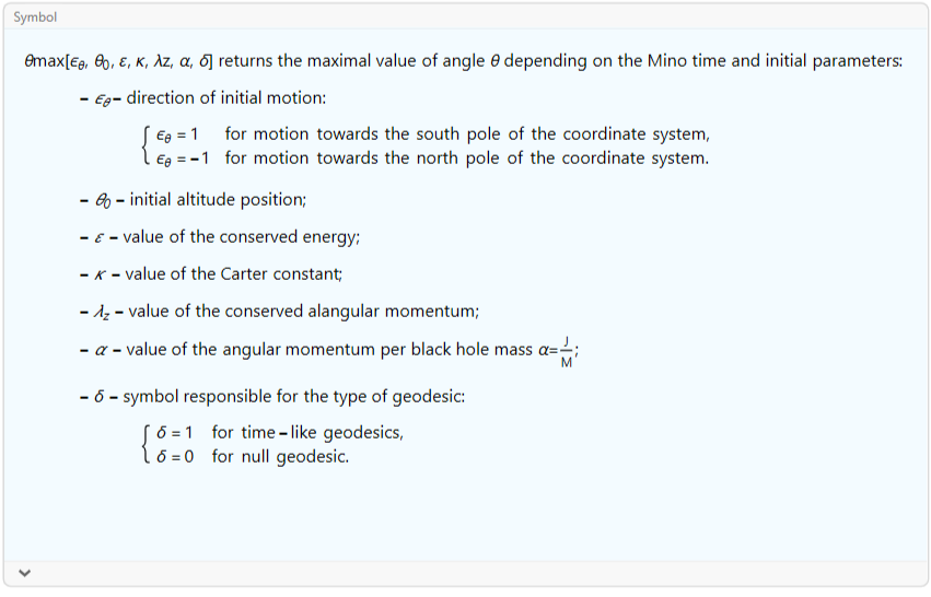
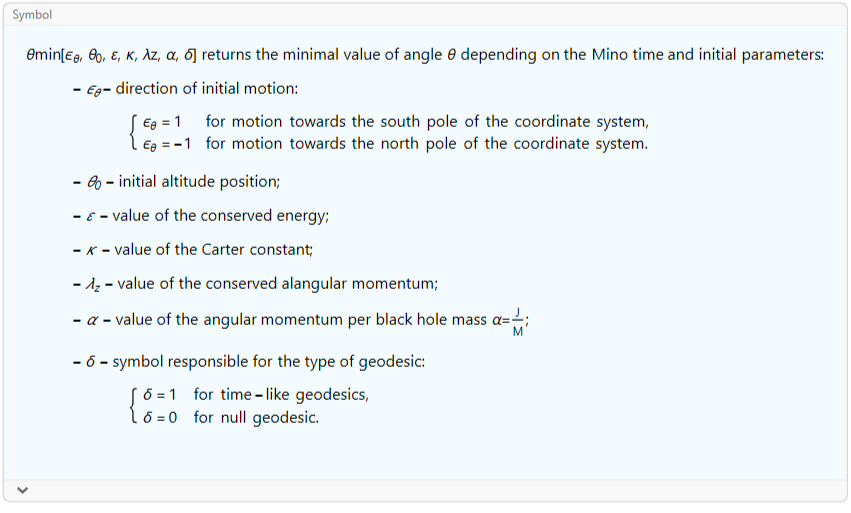
The package offers more features, such as
?θmax
?θmin
(Testy) In[]:=
?Fancylog
(Testy) Out[]=
Basic Examples
Basic Examples
Presenting a particle motion for given initial data is easy
Locations of Kerr horizons
Motion in the X-Y plane
Motion in the X-Y plane
Let us plot the motion in the X-Y plane
Motion in the X-Z plane
Motion in the X-Z plane
Marking the constraints
Marking the constraints
We can see that movement is restricted in θ. Using the θmax and θmin functions, we can draw these constraints.
Dynamic evolution
Dynamic evolution
In the case of movement in the X-Z plane, we can easily create a dynamic evolution with the change of the parameter s - Mino time. For motion in the X-Y plane, it is also feasible but considerably slower, as the φ coordinate relies on the complex logarithm derived from the ratio of two Weierstrass special functions. A more detailed explanation of this phenomenon can be found in the last section of this notebook.
First, we need to set some initial value of the parameter that we will change
Next, we create a slider that we will manipulate. We can also consider negative values of the Mino time, in other words, movement backwards in time.
Now, by changing the slider, we can see how the particle’s position changes in the plot below.
3D plot
3D plot
We can create a 3D plot with a sphere at the center, which has the external horizon’s radius for simplicity.
Proper time
Proper time
Fancylog
Fancylog
Conclusion
Conclusion
We’ve designed this package with the intention of providing utmost usefulness to our users. However, we acknowledge that there is always scope for improvement in our code. To make Fancylog faster, we are planning to upgrade its definition in the near future. We welcome any feedback or suggestions you may have, you can write to me here or in the comments.
CITE THIS NOTEBOOK
CITE THIS NOTEBOOK
Kerr Geodesics in Terms of Weierstrass Elliptic Functions
by Adam Cieślik
Wolfram Community, STAFF PICKS, December 21, 2023
https://community.wolfram.com/groups/-/m/t/3089149
by Adam Cieślik
Wolfram Community, STAFF PICKS, December 21, 2023
https://community.wolfram.com/groups/-/m/t/3089149