This notebook series is designed to introduce selected dynamic economic models to both advanced undergraduate and graduate students. Economists have relied on a series of economic models to better understand the otherwise highly complex causal relationship among many economic variables. Dynamic economic models set up by systems of either difference or differential equations are particularly useful in tracing the change in the quantity of unknown economic variables (e.g., the capital stock, demand for labor, aggregate output, etc.) and their interactions over time.
This notebook series aims to help students better understand the depth, usefulness, and limitations of major existing micro and macroeconomic models by demonstrating how we can use Wolfram Mathematica to replicate and reconstruct the core ideas and find dynamic solution of the model.
The model introduced in this notebook series include, among others, (1) the cobweb model of the quantity and price adjustment, (2) Keynes’s aggregate demand model, (3) Hicks’s ISLM model, (4) Samuelson’s investment accelerator model, (5) Kalecki’s investment delay model, (6) the predator-prey interaction model, (7) the epidemic model, (8) Ricardo’s three dimensional business cycle model, (9) Marx-Goodwin business cycle and growth model, (10) Smith’s and Ricardo’s growth model, (11) the Harrod-Domar growth model, (12) the Solow growth model, (13) the RBC model, (14) Romer’s new growth model, and (15) the circuit of capital model.
Kalecki’s investment-delay model
Introduction
Introduction
Kalecki introduces an internally generated self-perpetuating investment cycle associated with the time lag between investment decision-order, production of investment goods and the delivery and installation of this investment goods in the production of final consumption goods.
Starting from his famous profit equation, Kalecki links the investment process with both profit income and the existing capital stock. Because of the presence of time delay in between the investment order and the actual installation of the investment goods in the final goods producing sector, there emerges a self-propelling investment-led business cycle.
One unique feature in Kalecki’s business cycle model is that it relies on a mixed differential-difference equation tools. Most time delays in investment activities are expressed in terms of a fixed difference equation formulation, whereas the investment and capital stock accumulation process are expressed in terms of differential equations.
Aided by Gandolfo (2010)’s concise presentation of Kalecki model ( Kalecki 1933), this note reconstructs and visualizes Kalecki’s investment delay-led business cycle model. As an extension, this note also shows how we can trace the capital stock accumulation process in the consumption goods producing sector.
Preliminary: Capitalist profit income, investment spending, investment delay, and capital stock accumulation
Preliminary: Capitalist profit income, investment spending, investment delay, and capital stock accumulation
Capitalists’ gross profit income
Capitalists’ gross profit income
The total real income (profits) of capitalists, B, consists of capitalists’ consumption C and gross capital accumulation A.
B=C+A
(
1
)Capitalists’ consumption is a linear function of gross real profits with a constant fixed expenditure.
C=+λB
C
1
(
2
)where both and 0 < λ < 1 are positive constants.
C
1
From the two equations, we can obtain
B=+λB+A=+A
C
1
C
1
1-λ
(
3
)The delay in investment orders, production of capital goods, and delivery/installation of investment goods for final production
The delay in investment orders, production of capital goods, and delivery/installation of investment goods for final production
Kalecki assumes that there is an average time delay (“gestation lag”) in completing investment spending. Let θ denote this time delay. This gestation period of investment is the time interval between the decision to invest (investment order) and the delivery and installation of the finished capital goods. More precisely, we can determine the following three stages of investment process:
(1) Investment decision and order - Capitalists in the final consumption goods producing sector make a decision to increase their capital stock. They place an order for capital goods to the capital goods producing sector. Their decision can be made for either replacing a portion of the existing capital stock or for increasing the existing productive capacity (net addition to the existing capital stock). This decision and order must proceed the actual production and delivery of investment goods. Let us call this order I;
(2) Production of investment goods - The capital goods producing sector must incur a certain absolute amount of time to manufacture the ordered investment goods. This production corresponds to gross capital accumulation from a social point of view. Let us call it A;
(3) Delivery of finished investment goods and their installation in the final consumption goods producing sector of the economy. Let us call them L.
Given the assumption made above, we have the following relationship:
L(t)=I(t-θ)
(
4
)To find the relationship between I and A, let W(t) be the total amount in time t of unfilled investment goods orders. Since each order requires a period of time θ to fulfill it, and assuming that the production of capital goods to meet the order proceeds at an even pace (that is 1/θ of each order is executed per unit of time), it follows that the production of capital goods must be equal to (1/θ)W. Therefore,
A=(1/θ)W
(
5
)The variable W(t), the amount of unfulfilled order at time t equals the sum of all orders made in the interval (t-θ, t). Therefore,
W(t)=I(τ)τ
t
∫
t-θ
(
6
)Combining the two equations (5) and (6), we get:
A(t)=I(τ)τ
1
θ
t
∫
t-θ
(
7
)This equation means the output of capital goods at time t is equal to an average of the investment order placed in the interval (t-θ, t).
The change in the capital stock
The change in the capital stock
If we call K the capital stock, its first derivative with respect to time is its net increment, so that
K'(t)=L(t)-U
(
8
)The rate of change in capital stock is equal to the delivery of the finished capital goods to the final consumption goods producing sector (which is gross investment in this sector) minus the constant depreciation, U.
The investment function
The investment function
To close the model we need an investment function. There are two main factors that determine the investment behavior in Kalecki: The gross profit rate B/K and the money rate of interest, which he calls p. Therefore, the rate of investment is:
I/K=f,p
B
K
(
9
)From Kalecki’s point of view, the money rate of interest usually varies according to the general business conditions, which are represented by B/K, in the absence of external actions and except for situations of financial panic. Therefore, the investment function f can be rewritten as a function of B/K only. Since B, the capitalist gross profit income, is proportional to +A by equation (3), we can write
C
1
I/K=ϕ=ϕ+A≃m+A-n
B
K
C
1
K
C
1
K
(
10
)where ϕ is an increasing function, and both m and n are linearized constants (m, n > 0). Therefore, investment is a positive function of (prospective) profit income but a negative function of the existing capital stock.
I=m(+A)-nK
C
1
(
11
)The Kalecki’s business cycle model and its analytical solution
The Kalecki’s business cycle model and its analytical solution
The basic equations of the model
The basic equations of the model
To collect all the crucial equations in Kalecki, we have:
L(t)=I(t-θ)
(
12
)A(t)=I(τ)τ
1
θ
t
∫
t-θ
(
13
)K'(t)=L(t)-U
(
14
)I=m(+A)-nK
C
1
(
15
)The mixed differential-difference equation
The mixed differential-difference equation
Differentiating both equation (13) and (15), we get:
A'(t)=
I(t)-I(t-θ)
θ
(
16
)I'(t)=mA'(t)-nK'(t)
(
17
)Combining the equation (12) and (14), we get:
K'(t)=L(t)-U=I(t-θ)-U
(
18
)Substituting the equation (16) and (18) into the equation (17), we have:
I'(t)=mA'(t)-nK'(t)=(I(t)-I(t-θ))-n(I(t-θ)-U)
m
θ
(
19
)To simplify further, let J(t) be the difference I(t) - U, that is net investment. Its derivative J’(t) = I’(t) since U the depreciation is constant. Using this identity, we can rewrite the equation (19) into
J'(t)=(J(t)-J(t-θ))-n(J(t-θ))⟺θJ'(t)=mJ(t)-mJ(t-θ)-θnJ(t-θ)⟺θJ'(t)-mJ(t)+(m+θn)J(t-θ)=0.
m
θ
(
20
)The last equation in (2) is a mixed differential-difference equation.
A numerical solution and visualization of net investment
A numerical solution and visualization of net investment
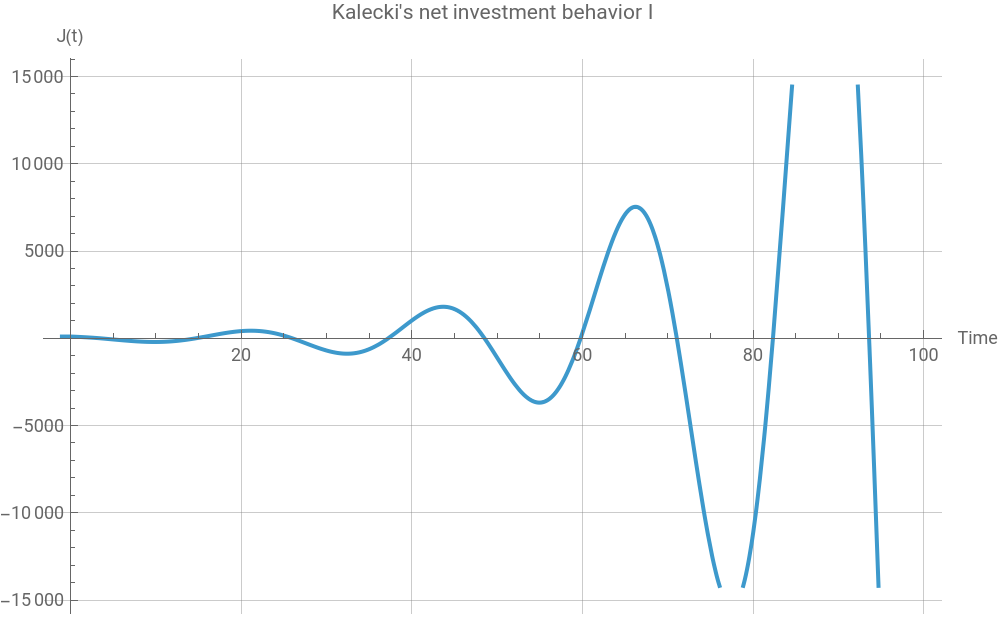
A static visualization with fixed parameters
A static visualization with fixed parameters
Suppose we have the following arbitrary parameter values:
In[]:=
Clear[J,t,m,n,θ,sol1];θ=4(*delaybetweeninvestmentorderanddelivery*);m=0.8(*investmentsensitivitytogrossprofit*);n=0.2(*investmentsensitivitytotheexistingcapitalstock*);sol1=NDSolve[{θJ'[t]-mJ[t]+(m+θn)J[t-θ]==0,J[t/;t≤0]==100},J[t],{t,-1,100}]
Out[]=
J[t]InterpolatingFunction[t]


In[]:=
Plot[Evaluate[J[t]/.sol1[[1]]],{t,-1,100},PlotLabel->"Kalecki's net investment behavior I",AxesLabel->{"Time","J(t)"},ImageSize->500,GridLines->Automatic]
Out[]=
An interactive visualization
An interactive visualization
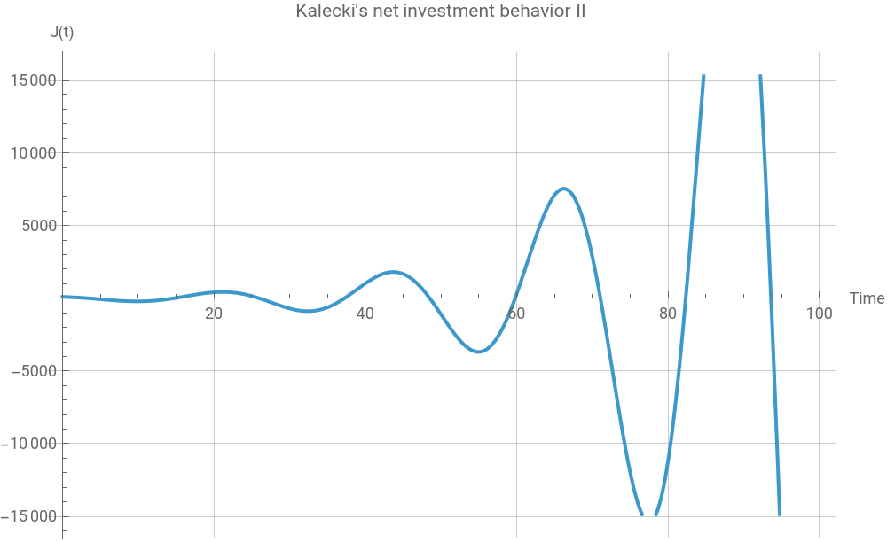
We can also create an interactive chart using the following syntax:
In[]:=
Clear[J,t,m,n,θ,sol2];sol2=ParametricNDSolve[{θJ'[t]-mJ[t]+(m+θn)J[t-θ]==0,J[t/;t≤0]==100},J,{t,0,100},{θ,m,n}]
Out[]=
JParametricFunction

In[]:=
Manipulate[Plot[Evaluate[J[θ,m,n][t]/.sol2],{t,0,100},PlotLabel->"Kalecki's net investment behavior II",AxesLabel->{"Time","J(t)"},GridLines->Automatic,ImageSize->500],{{θ,4},1,12},{{m,0.8},0.6,0.9},{{n,0.2},0.1,0.4},SaveDefinitions->True]
Out[]=


An interactive visualization of net investment and the capital stock
An interactive visualization of net investment and the capital stock
As a final step, let us create an interactive chart that shows how net investment and the capital stock interact with one another as time goes by. From the equations from (18) through (20), we know that the capital stock at time t is nothing more than an integral of net investment. In a differential equation form, we can write K’(t) = J(t).
Using this identity, let us interactively visualize the solution curve of both J(t) and K(t) and their interaction over time.
Conclusion
Conclusion
This note aims to replicate the core ideas of Kalecki’s investment delay-led business cycle model, while tracing the corresponding capital stock accumulation process. Kalecki’s commonsense ideas that it takes some time for entrepreneurs-capitalists-manufacturers to complete their investment projects require solving a mixed difference-differential equation problem. The time delay among the investment order, production of investment goods, and the delivery/installation of this productive equipment in the final consumption goods producing sector inevitably introduces nonlinearity in the system. The longer the delay, the more the fluctuation in net investment and accumulation of capital stock.
Reference
Reference
◼
Giancarlo Gandolfo, Economic Dynamics, Berlin and Hidelberg: Springer-Verlag, 2010, pp.582-89.
◼
Michal Kalecki, “Outline of a Theory of the Business Cycle,” in Studies in the Theory of Business Cycles, London: Routledge, 1966 [1933].
CITE THIS NOTEBOOK
CITE THIS NOTEBOOK
Introduction to dynamic economic models
by Hee-Young Shin
Wolfram Community, STAFF PICKS, December 2025
https://community.wolfram.com/groups/-/m/t/3596138
by Hee-Young Shin
Wolfram Community, STAFF PICKS, December 2025
https://community.wolfram.com/groups/-/m/t/3596138