CITE THIS NOTEBOOK: System dynamics and Hooke's law by Ricardo Martinez-Lagunes. Wolfram Community OCT 25 2022.
The diagram shown below illustrates Hooke’s law with a set of interconnected stocks and flows. Stocks are represented by boxes and flows are represented by arrow-headed pipes with a faucet in the middle.
The figure shows the following relationships: a spring exerts an opposite force (acceleration of mass) directly proportional to the distance of the mass from rest conditions. The force of the spring is expressed as an acceleration opposite to the direction the mass is moving. Therefore, the speed is reduced by the acceleration, which is proportional to the distance. On the other hand, the distance is changed by the speed of the mass.
The figure shows the following relationships: a spring exerts an opposite force (acceleration of mass) directly proportional to the distance of the mass from rest conditions. The force of the spring is expressed as an acceleration opposite to the direction the mass is moving. Therefore, the speed is reduced by the acceleration, which is proportional to the distance. On the other hand, the distance is changed by the speed of the mass.
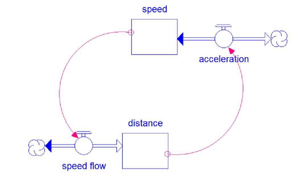
The diagram can be translated into a system of first order differential equations as follows:
{speed'[t]-k*dist[t],dist'[t]speed[t],speed[0]0,dist[0]5}
The equations can be interpreted as follows:
1. The derivative of speed is directly proportional to the distance of the object from the equilibrium point.
2. Speed is the derivative of distance from the equilibrium point.
3. At time = 0, initial condition, speed = 0 and distance = 5.
In other words, the flow of acceleration changes stock of speed. The stock of speed is at the same time the flow that changes the stock of distance. The floowing graph shows speed and distance through time.
In[]:=
Manipulate[Plot[Evaluate[{speed[t],dist[t]}/.NDSolve[model[k,d],{speed,dist},{t,0,30}],{t,0,10}],AxesOrigin{0,0},PlotRange{Automatic,{-30,30}},PlotLegendsPlaced[{"Speed","Distance"},Above],ImageSizeLarge],{{k,14,"Stiffness of the spring "},1,20,1,Appearance"Labeled"},{{d,5,"Intital distance "},1,10,1,Appearance"Labeled"},Initialization(model[k_,initdist_]:={speed'[t]-k*dist[t],dist'[t]speed[t],speed[0]0,dist[0]initdist}),SaveDefinitions->True]
Out[]=


Written by Ricardo Martínez-Lagunes for educational purposes D.R. 202228 August 2022